Latest Posts From Wasim Akram

Safety Stock Safety stock acts as a buffer to ensure that a company can meet customer demand even during unexpected fluctuations in demand or lead time. ...

Here's an overview of a private sub in VBA. What Does Private Sub Mean in Visual Basic? A private sub refers to a subroutine or method that is ...

Excel VBA provides a powerful solution for converting text to columns with multiple delimiters. By leveraging VBA macros, you can automate the process of ...

Issues with Excel Comments: Knowledge Hub Comments in Excel Far Away from Cell Excel Comment Only Showing Arrow Comments Are Not Displaying ...

How to Launch the VBA Editor in Excel Utilizing the Module Tool: Open your workbook and click Visual Basic in the Developer tab. Choose ...

Excel slicers with search functionality offer a user-friendly way to filter and navigate data within Excel. By incorporating a search feature, users can ...
The Power Query tool can be used to export .xlsx and .txt file inside a folder and subfolder list to Excel. Step 1 - Choose a Folder from the Data ...
How to Launch the VBA Editor in Excel Utilizing the Module Tool: Open your workbook and select Visual Basic in the Developer tab. Choose ...
The Least Squares Regression Line - A Statistical Tool for Analyzing Relationships The least squares regression line is a widely used statistical method for ...

A back-to-back stem and leaf plot in Excel is a type of data visualization tool that helps you compare two sets of data on the same graph. It shows the ...

In Microsoft Excel, deselecting means removing the active selection of cells or a range of cells in the worksheet. Deselecting cells can be useful when you ...
Method 1 - Find the Coefficient of Determination from the Correlation Coefficient 1.1 Using Arithmetic Formula Steps 1: Multiply the independent and ...
What Is an Excel VBA MsgBox? The Excel VBA MsgBox is a built-in function in Microsoft Excel's Visual Basic for Applications (VBA) programming language, which ...

Here's an overview of making a time series graph in Excel. How to Make a Time Series Graph in Excel: 3 Useful Methods Method 1 - Making a ...
Example 1 - Customizing an Input Box with a Custom Prompt Message Steps: After opening a new module, insert the following code and run it by hitting the ...
- « Previous Page
- 1
- 2
- 3
- 4
- …
- 10
- Next Page »
See Our Reviews at


Dear FODAY,
Thank you for your response. As per your query-
1. You can create a Pie Chart to visualize the sales from the “Insert” option.
Imagine a dataset with multiple Bakery Products and their Total Sales. Now we will create a pie chart using the information from the dataset.
First, select the products and total sales column and then press “Recommended Chart” from the “Insert” option.
Second, from the new dialog box choose “Pie Chart” and press OK to continue.
Finally, within a moment your final pie chart will be in your hands showing sales of multiple products.
2. As per your second query-
We will use the IF function to calculate the “10%” discount price if the sales of cake is more than 100.
To do that choose a cell (G5) and write the following formula down-
=IF(E5>100,(D5-(D5*0.1)),D5)Hence, hit Enter and the final output will be in your hands.
3. Now coming to the last query you wanted to use the data validation for ladies with only 5 letters in their name. Well, below I have shared the simplest solution.
Suppose we have a dataset with some Lady Names. Now we will use data validation for the name list.
First, selecting the names from the list click the “Data Validation” option from the “Data” feature.
Second, click “Settings” and choose criterias according to the screenshot and press OK to continue.
Finally, we have applied data validation over the name list. To check try editing any names not fulfilling the condition and you will get a notification about “This Value doesn’t match the data validation restrictions defined for this cell.”
Dear AJ,
Thank you for your response.
There are a few potential issues that could prevent this code from working properly-
1. Make sure that the worksheet module contains the correct event handlers. To do this, right-click on the worksheet tab in Excel and select “View Code”. Then, make sure that you have pasted the code into the correct module, which should be named something like “Sheet1 (Sheet1)”.
2. Check that the password used to protect and unprotect the workbook is correct and does not contain any typos. In this case, the password is set to “”123″”, but you can change this to any other password of your choice.
3. Ensure that the workbook is not already protected by another password. If the workbook is already protected, you may need to unprotect it first before running this code.
If none of the above solutions work, you may need to provide more context or information about the specific error message or issue you are encountering when trying to run this code.
Thanks
Wasim Akram
Exceldemy Team
Hello jean,
Thank you for sharing your problem with us!
In order to calculate the participation percentage, you can follow the instructions below.
1. Simply choose a blank cell.
2. Insert the following formula:
=COUNTIF($C$5:$C$25, E5)/COUNTA($C$5:$C$25)Thus you can calculate the participation percentage.
Note:
1. The formula you used did not work because you did not lock the cell range using absolute reference.
2. Another reason is don’t leave the cells blank for the choosen cell range.
Dear Betty Domowski,
Thank you for sharing your problem. As you already know how to get rid of these lines but to stop them from coming back there is no other alternative except using the Remove Arrows option from the Formulas tab. Please check the image below.
Hope you found your solution you are looking for.
Regards
Wasim Akram
Exceldemy
Dear vishal saini,
Thank you for your response.
Here I have shared a solution using VBA code to protect a worksheet in the manner you are looking for.
First, opening the VBA window you need to put the following code in the This Workbook section. Don’t forget to change the sheet name according to your sheet.
Next, insert the below code in your worksheet. You can change the password from the marked section.
Finally, you can protect your worksheet in the manner where you can add data and after saving the data you can’t delete the same until you don’t save.
Thanks
Wasim Akram
Exceldemy Team
Hi Farhan,
Hope you are doing well.
Here Jacob and Ben are sales representative working in both night and day shifts.
In order to calculate their day and night shift from the list for each we used a simple formula using the COUNTIFS function.
First, the COUNTIFS function counts the number of cells in the cell range ($C$5:$C$92) matching the value in cell (K23) which indicates sales representative Ben.
Next, it also match the value in cell (L22) within the cell range ($D$5:$D$92).
As a result, we will get the result counting total number of day shifts attended by Ben.
Similarly, we can calculate the total number of shifts attended by Jacob.
Hope you found the answers for your submitted queries.
Regards
Wasim Akram
ExcelDemy
Dear Anita,
Thank you for the comment. We really appreciate your response for sharing with us.
The currency sign not appearing in Excel may be due to the values are stored as text in your spreadsheet. When values are stored as text, you need to convert those as numbers and then change the format to currency to get your desired currency format. You can follow the below instructions to learn about this technique.
First, choose the cells (D5:D12) and click the error icon following the image below.
Next, choose Convert to Number option from the list.
As the numbers are now converted as number, now press CTRL+1 to visit the Format Cells feature to add currency symbol.
From the Format Cells window, choose Currency from the left pane, select your desired currency symbol and hit OK.
As a result, you will get the currency sign added in your worksheet.
If you are still having problem with the currency symbol, then you can share your workbook with us. We will check and solve the problem.
Thanks & Regards
Wasim Akram
Team Exceldemy
Dear Brenda,
Thank you for your comment.
In order to create a pie chart you don’t need to create a pivot table. But if your data have duplicate values then you must create a table to group those data and then create a pie chart. Otherwise the duplicate value will not group together. Because there’s no direct command or pivot pie chart in Excel to group data.
There’s Pivot chart feature by which you can group data from pivot table fields and that is a column chart not pie chart. That’s why you need to create a table first and then create the pie chart.
We’ll really appreciate your response If you have any alternative solution and share with us.
Thanks & Regards
Wasim Akram
Team Exceldemy
Dear Ben,
Thank you for your comment. We really appreciate you for contacting with us.
In order to insert multiple rows of data, you can try the below VBA code.
Using the Array statement inside the VBA code, you can add as many rows you want inside your table.
Thanks & Regards
Wasim Akram
Team Exceldemy
Dear Yogiraj,
Thank you for your comment.
You are absolutely right about your opinion regarding its use.
By creating equation from data points you can also see the difference between the plotted and actual data points.
Thanks
Dear TAYFOON,
Thank you for your response.
If you want to see the arguments as “RETAILPRICE(Price1,Price2,Divisor)”.
Then follow the instructions below-
1) In the module Place the following code-
Public Function RETAILPRICE(Price1, Price2, Divisor)

RETAILPRICE = (Price1 + Price2) / Divisor

End Function
2) Then go to your worksheet and type “=RETAILPRICE(” and after that press Ctrl+Shift+A to get the arguments just as you want.
Hope you found your solution. Thanks!
Dear MIKE WELLS,
Thanks for your response.
There are several reasons behind this “Source Validates to an error” occurring. You can solve them efficiently providing the correct data inside the string.
Reason: The source validates that an error can occur if the source to which the formula is applied demonstrates an error. Thus the final statement stands to whether the formula is not correct or the formula refers to data returning an error.
Solve: To solve this problem, you have to provide correct data or change the formula.
From our dataset, suppose we are having trouble with the “Source Validates to an error“. This error is occurring due to the blank cell (E4). As the INDIRECT function converts a string into an actual reference thus finding the reference cell (E4) blank it’s showing an error. Check the following screenshot.
In order to solve this just put the same text from the list in the reference cell and you won’t find any more errors further.
Other reasons behind this “Source Validates to an error” might happen-
a) The applied formula is not the proper formula to find the references.
b) Put exact names from the list to the reference list to avoid errors.
Hope you will find your solution with this reply. If you are still having problems, don’t hesitate to let us know below. We are always here with you to solve your problems. Thanks!
Dear FLEET,
Thank you for your response.
The answer for the intersection of “Laptop” and “China” will be “$63,800”.
The SUMPRODUCT function returns the sum of an array from an argument. With the intersection between “China” and Laptop” within the cell range we got two outputs which are “$56,000” and “$7,800”. Thus summing the total value with the SUMPRODUCT function stands to “$63,800”.
You can check the screenshot below.
We have also attached a worksheet with our article. You can practice the formula there, too. Thanks!
Dear SWAROOP,
A syntax error occurs due to misspelling or missing code. Mostly, due to not specifying the condition and not putting closing brackets. You can check the VBA editor which will help you identify the problems. You can try applying the code in a new worksheet to find your solution.
In addition, if you are applying VBA code with your own workbook data, don’t forget to change the ranges. Check the below screenshot. Thanks!
Dear ERIC CHARLES BAUMGARDNER,
In order to enter your own workbook value into the code, you need to change the ranges inside the code. Check the following screenshot. Thanks!
Dear RUBY,
Here is the solution you are looking for.
Suppose you have a dataset with conditional formatting applied in the list.
First, select all the cells (C2:C11) from the column and click the “Filter” option from the “Data” ribbon.
Now press the “Filter icon and choose “Filter by Color”. Hence choose your cell color.
Thereafter, you will get to see only the cells with the selected colors. Let’s calculate the total sum now. To do so, choose a cell (C13) and writhe the following formula down-
=SUBTOTAL(109,C3:C11)
Finally, you will get the sum value for the colored cells only.
If you are still facing problems then you can read this article – How to Sum Colored Cells in Excel
Thanks!
Dear Jamil,
Using conditional formatting you can search for a specific text and color them according to your choice. Follow the instructions below.
Suppose we have a dataset of some countries’ names in cells (B3:E9). Now we are going to color a specific text (United States) from the list.
First, select all the cells and click the “Text that contains” option from the “Conditional Formatting” feature.
Second, put your desired text and choose a color of your choice. Gently, press OK.
Finally, we have successfully highlighted a certain text from the list.
Hope you got the solution you are looking for. If you still having problems then check the link below. Thanks!
Highlight Cells Based on Text
Dear KOLAPALLI PAVAN KUMAR,
The output you are looking for can be achieved using the COUNT function in excel. Here the COUNT function counts the cell number given in the string.
Apply the following formula-
=COUNT(C2:C8)You can check the screenshot below-
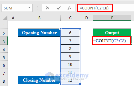
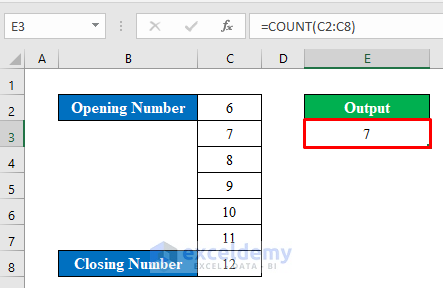
First, select a cell (E3) to apply the formula.
Second, press Enter to get the desired output.
Hope you got your solution. If you still didn’t get it, check out the article below-
The Different Ways of Counting
Thanks!
Dear DON_1234567,
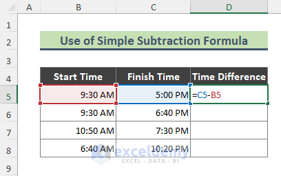
You can use the simple subtraction formula to calculate the difference between two times.
You can use the formula below-
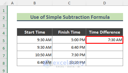
=C5-D5Check out the screenshot below-
If you are still not getting the result. Then change the cell format to time.
You can visit the below article to learn more. Thanks!
Calculate Difference Between Two Times