Latest Posts From Tanjima Hossain
![[Fixed!] NAME Error in Excel (7 Reasons with Solutions)](https://www.exceldemy.com/wp-content/uploads/2021/12/1-name-error-in-excel-2.png?v=1697520201)
Excel is a powerful tool widely used for data analysis, organization, and reporting. While working with formulas and functions, you may come across a common ...
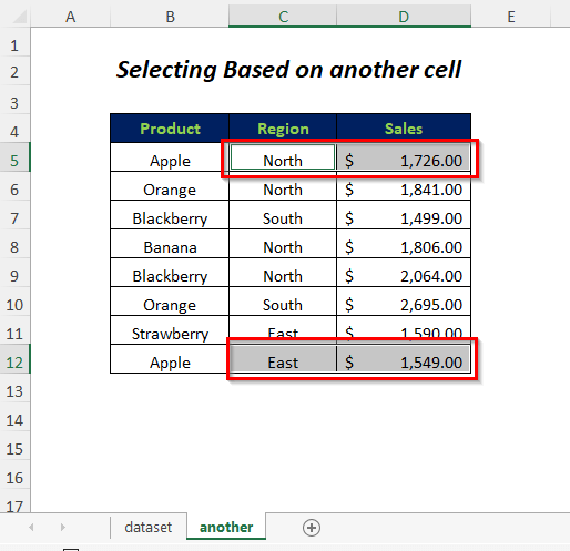
Method 1 - Selecting Range Based On Another Cell Value We will select the cell range in the Region and Sales column based on the string Apple in the Product ...

We have a dataset of a company to demonstrate the ways of using a dynamic range in VBA. Method 1 - Select Cells Containing Values Through UsedRange ...

In this article we will demonstrate a variety of ways to use the VBA Range Offset. Here is an overview. 11 Suitable Ways to Use VBA Range Offset To ...

Here's an overview of using Conditional Formatting for multiple conditions. We have the two data tables, which we'll format. The first table has the ...

Here's the overview of the functions we'll use today and how they highlight cells or rows based on dates or ranges. We have a data table with the Sales ...
Here's an overview of using Conditional Formatting based on another cell range. We have two data tables. The first table has Sales values for different ...
Consider a dataset about some products of a company. We will check whether specific values in the Product column exist. Method 1 - Using Find & ...

Here's an overview of using slicers to filter a table by specific value. Read on to learn more. Split Excel Sheet into Multiple Sheets Based on ...

Download the Workbook VBA Find and Replace. xlsm How to Find and Replace Using VBA - 11 Ways We will use the following table which has ...
Suppose you have the following dataset: Method 1 - Find an Exact Match in a Range of Cells Steps: Press Alt+F11 on your keyboard to open the ...
In this article, we will demonstrate how to use Excel VBA to find the position of a substring in a string, to extract data using this substring, and to change ...
The sample dataset showcases Fruits, Region, Vendor, Quantity, Delivery Date and Sales. You want to sum Sales or Quantity values based on different ...

We have two datasets: a company's Record of Sales, and the records for construction company X, containing different projects and their costs. ...
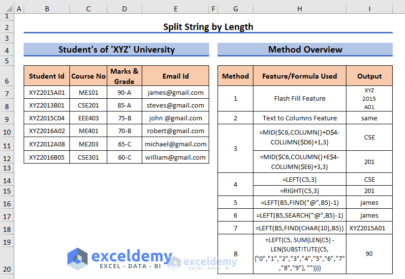
This is an overview. The dataset showcases students’ records. Method 1 - Using the Flash Fill Feature to Split a String by Length Student Id ...
See Our Reviews at


Hello GURI,
You can download the Excel and PDF files free of cost just by providing your valid email address. To get the files go to the “Download Excel Formulas Cheat Sheet PDF & Excel Files” section of this post and enter your email address. Then check your email immediately after to get the download links.
Best Regards
ExcelDemy
Hello MS,
The link will be sent to your Email Id which you will use to fill up the form in the download section of this article.
Please provide your valid Email address in the form of the download section.
Thanks
ExcelDemy
Hello Excel Guru,
Thanks for your comment. The article has been updated, so you can try the code now easily for January month also. And the previous code was not buggy obviously, it was used for another purpose and so it also gave results.
Thanks
ExcelDemy
Hello Alphonse,
Thanks for your appreciation.
You can try the code below to count number of Mondays for a month of a year
• Then, type the function name and enter the month name and year to count Mondays.
As a result, we are getting 5 which represents Mondays of January 2023.
Best Regards
ExcelDemy
Hello Rupert,
Sorry to hear about your trouble. But this code is working for use. You can try the following steps to run this code successfully.
• You can Right-click on the sheet name to open the code window for writing the code.
• After writing down the code in the window when you will try to run it, you will see the sheet name before the sub procedure name like below.
• After running the code in this way, we got the following result.
• Moreover, you can try to remove Option Explicit from the first line of the code.
Hope this will work for you.
Best Regards
ExcelDemy
Hello Ali,
Hope you are doing well. I tried to create a custom format with number/text/number for numeric values like 14002502.
• After opening up the Format Cells dialog box, type the following format in the Type area under the Custom tab.
#### "/Pound/" ####Here, #### represents four digits before and after the text. Here, I used “/Pound/” as the text part within inverted commas.
• After pressing OK, you will get the following results.
Best Regards
ExcelDemy
Hello BOB,
We can open our password-protected files using the stated procedures. I have tried this way right now, and it worked. I could also change the values of worksheets.
But if you encrypt your file with a password like the following figure, then it may not work for you.
Thank You
Tanjima Hossain
Hello Michael,
Hope you are doing well. Here, I have the following dataset containing 3 columns where we have some products. After combining all of the columns into a column we will clean up all of the empty cells.
• Write down the following code in a module.
• Press F5.
Then, you will get the following input box.
• Select the range of cells containing texts and press OK.
Later, another input box will appear.
• Select the whole data range containing all the blank cells.
• Press OK.
In this way, we combined all of the columns in the first column and deleted the rest of the cells.
Best Regards
Tanjima Hossain
Hello Nilsen,
Sorry, this formula will not work for copying both a comment and a picture as a comment. You have to copy only the text strings if you want to paste them as comments. But if you want to copy the contents as cell value then try the previous code.
Stay in touch with ExcelDemy.
Thanks
Tanjima
Hello MICHAEL,
Thanks for your inquiry. Actually, the formula used in Method-1 has been updated to use in Method-3 for behaving differently from Method-1. In Method 1 we tried to combine two columns by adding another column after the ending of one column. But in Method-3 it was the intent to join 2 columns by adding the cell contents row-wise. If you need to add the columns serially then please follow the previous 2 methods.
Thank you
Tanjima Hossain
Hello NILSEN,
Hope you are doing well. Here, I have inserted a comment to cell B3 and in this comment, we have some text along with an image. So, using a VBA code I will show the process of extracting the image and texts in different cells.
• Type the following code.
In the figure above, look at the highlighted portions which you may want to change.
Set Range = .Parent.Offset(0, 4)will insert the image in a cell which is 4 columns right to the main cell B3 and.Parent.Offset(0, 3)will insert the texts in a cell which is 3 columns right to the main cell B3.• Press F5.
Then, we transferred the texts and images from the comment into different cells.
Best Regards,
Tanjima Hossain
ExcelDemy
Hello JORDAN,
Hope you are doing well! As per your requirement, I am considering the following scenario where in a table I have two lists of products with which I will compare the products in the Order List column. I will use a formula that will match a product from the Order List column with products from the Product List 1 column, for matches, the name of the product will return. Otherwise, the formula will search for matches in the Product List 2 column and will return the product name if any matches are found. Otherwise, we will get “No Match”.
• Enter the following formula in cell F4.
=IF (COUNTIF ($B$4: $B$10, E4)>0, E4, IF (COUNTIF ($C$4: $C$10, E4)>0, E4, "No Match"))• Drag down the Fill Handle tool.
Finally, we are having Green Apple and Kiwi as they appear in the Product List 2 column, and Banana as it appears in the Product List 1 column.
Best Regards,
Tanjima Hossain
ExcelDemy
Hello ERFLING,
Thanks for your valuable suggestion. But you can take a look at Section 7 of this article which may align with this requirement.
Thanks
Tanjima Hossain
ExcelDemy
Hello SEAN,
Here, we have listed the following tasks in a sheet which we will classify according to their importance and urgency.
• For creating drop-down lists for each of the cells in range C5:D12, we have opened the Data Validation dialog box.
• In the Source box, type High, Medium, Low.
Then, we selected the following values for the tasks in the Task sheet.
In another sheet named Matrix, we have created the following template.
• For the portion of High Important and High Urgent use the following formula in cell D5, press ENTER, and use the AutoFill feature up to cell D8.
=IFERROR(INDEX(Task!$B$5:$B$12,SMALL(IF((LEN(Task!$B$5:$B$12)<>0)*(Task!$C$5:$C$12="High")*(Task!$D$5:$D$12="High"),ROW(Task!$B$5:$B$12)-ROW(Task!$B$4),""),ROW(Task!B5)-ROW(Task!$B$4))),"")• For the portion of High Important and Medium Urgent use the following formula in cell F5, press ENTER, and use the AutoFill feature up to cell F8.
=IFERROR(INDEX(Task!$B$5:$B$12,SMALL(IF((LEN(Task!$B$5:$B$12)<>0)*(Task!$C$5:$C$12="High")*(Task!$D$5:$D$12="Medium"),ROW(Task!$B$5:$B$12)-ROW(Task!$B$4),""),ROW(Task!B5)-ROW(Task!$B$4))),"")• For the portion of High Important and Low Urgent use the following formula in cell H5, press ENTER, and use the AutoFill feature up to cell H8.
=IFERROR(INDEX(Task!$B$5:$B$12,SMALL(IF((LEN(Task!$B$5:$B$12)<>0)*(Task!$C$5:$C$12="High")*(Task!$D$5:$D$12="Low"),ROW(Task!$B$5:$B$12)-ROW(Task!$B$4),""),ROW(Task!B5)-ROW(Task!$B$4))),"")• For the portion of Medium Important and High Urgent use the following formula in cell D9, press ENTER, and use the AutoFill feature up to cell D12.
=IFERROR(INDEX(Task!$B$5:$B$12,SMALL(IF((LEN(Task!$B$5:$B$12)<>0)*(Task!$C$5:$C$12="Medium")*(Task!$D$5:$D$12="High"),ROW(Task!$B$5:$B$12)-ROW(Task!$B$4),""),ROW(Task!B5)-ROW(Task!$B$4))),"")• For the portion of Medium Important and Medium Urgent use the following formula in cell F9, press ENTER, and use the AutoFill feature up to cell F12.
=IFERROR(INDEX(Task!$B$5:$B$12,SMALL(IF((LEN(Task!$B$5:$B$12)<>0)*(Task!$C$5:$C$12="Medium")*(Task!$D$5:$D$12="Medium"),ROW(Task!$B$5:$B$12)-ROW(Task!$B$4),""),ROW(Task!B5)-ROW(Task!$B$4))),"")• For the portion of Medium Important and Low Urgent use the following formula in cell H9, press ENTER, and use the AutoFill feature up to cell H12.
=IFERROR(INDEX(Task!$B$5:$B$12,SMALL(IF((LEN(Task!$B$5:$B$12)<>0)*(Task!$C$5:$C$12="Medium")*(Task!$D$5:$D$12="Low"),ROW(Task!$B$5:$B$12)-ROW(Task!$B$4),""),ROW(Task!B5)-ROW(Task!$B$4))),"")• For the portion of Low Important and High Urgent use the following formula in cell D13, press ENTER, and use the AutoFill feature up to cell D16.
=IFERROR(INDEX(Task!$B$5:$B$12,SMALL(IF((LEN(Task!$B$5:$B$12)<>0)*(Task!$C$5:$C$12="Low")*(Task!$D$5:$D$12="High"),ROW(Task!$B$5:$B$12)-ROW(Task!$B$4),""),ROW(Task!B5)-ROW(Task!$B$4))),"")• For the portion of Low Important and Medium Urgent use the following formula in cell F13, press ENTER, and use the AutoFill feature up to cell F16.
=IFERROR(INDEX(Task!$B$5:$B$12,SMALL(IF((LEN(Task!$B$5:$B$12)<>0)*(Task!$C$5:$C$12="Low")*(Task!$D$5:$D$12="Medium"),ROW(Task!$B$5:$B$12)-ROW(Task!$B$4),""),ROW(Task!B5)-ROW(Task!$B$4))),"")• For the portion of Low Important and Low Urgent use the following formula in cell H13, press ENTER, and use the AutoFill feature up to cell H16.
=IFERROR(INDEX(Task!$B$5:$B$12,SMALL(IF((LEN(Task!$B$5:$B$12)<>0)*(Task!$C$5:$C$12="Low")*(Task!$D$5:$D$12="Low"),ROW(Task!$B$5:$B$12)-ROW(Task!$B$4),""),ROW(Task!B5)-ROW(Task!$B$4))),"")Note:
Here, we have used the sheet name Task in all our formulas, if you have any other sheet name, then put this name in the formulas.
Regards
Tanjima Hossain
Hello JAN T,
Hope you are doing well. I think by following the below-stated procedures you can make your code work.
• After going to your VBE window, go to the Tools tab >> References option.
Then, the References – VBAProject window will appear.
• Check the following options.
o Microsoft Scripting Runtime
o Microsoft WinHTTP Services, version 5.1
• Press OK.
• Now, type the following code.
Make sure to add a third argument in your code and use it in the indicated place.
• Finally, go to your sheet and use the following function.
One thing to mention is that make sure to use a valid API address, otherwise, you will get an error.
Regards
Tanjima Hossain
Hello MAREK,
Hope you are doing well. As far as I understand, you wanted to change the position of the background images or hide any row with these images. I think we can do these works as I demonstrated below.
Firstly, in Section 1, you can move the background image by clicking on the cell and then dragging it to your desired position.
• Here, we have dragged the image beside the cell and changed the text written also in this cell.
• In Section 3, you can move the image along with the text to any position by only clicking on this cell and then dragging it.
In this way, we have changed the position.
• Later, we also changed the text.
• If you want to hide any row, then just click on this row, and then Right-click.
• Select the Hide option.
Eventually, we have hidden our desired row.
Hello PEDRO,
As per your question, I will try to show an easier way to remove a specific value from a row. Here, we have the specific text “Furniture” in three rows which we will remove from these rows.
• Go to the Home tab >> Find & Select dropdown >> Replace option.
Then, you will have the Find and Replace dialog box.
• Type Furniture in the Find what box, and blank in the Replace with box.
• Click on Replace All.
Then, a message box will notify you about the number of replacements.
In this way, we have removed Furniture from three rows.
If you want to remove this specific text from a specific row only, then before doing the stated procedures just select that specific row.
Best Regards,
Tanjima Hossain
Hello ANTHONY,
If your second to the last row is situated in Row 11, then you can use the following formula.
=INDEX(‘[Sales.xlsx]Dataset’!$A$11:$H$11,COUNTA(‘[Sales.xlsx]Dataset’!$A$11:$H$11))
You have to just change the reference according to the position of your desired row.
Best Regards
Tanjima Hossain
Hello STEFAN,
We can open our password-protected files using the stated procedures. I have tried this way right now, and it worked. I could also change the values of worksheets.
But if you encrypt your file with a password like the following figure, then it may not work for you.
Thank You
Tanjima Hossain
Hello DARREN,
Hope you are doing well. So, to solve your issue you can follow the stated procedures below.
Here, we have the following three sheets- April, May, June, etc. Using a VBA code, we will print all these sheets into PDF format separately.
• Type the following code in your Visual Basic Editor window.
Finally, you will get the PDF files in your designated folder.
Also, the PDF files will be opened automatically.
I hope these steps will give your desired results.
Thank you
Tanjima Hossain
Hello MRA,
Thanks for your appreciation. Stay with us always.
Best Regards
Tanjima Hossain
Hi RICK,
The maximum number of sheets in a workbook is 255. So, if you have values in rows on basis of which you will split your sheet for more than 255 rows, then you may face a problem.
Hello KEVIN,
Hope you are doing well. You can follow the procedures below to get the address of the rightmost cell.
Here, we have taken the following dataset into our consideration. Suppose, the user selected the header of the dataset which is A3:G3.
• Go to the Developer tab >> Visual Basic option to open the Visual Basic Editor window.
• Use the following code.
• Press F5.
Then, you will get the following message with the rightmost cell of the selected range $G$3.
Hello DOUG,
Hope you are doing well. You can follow the stated technique below to keep the pivot tables intact in a worksheet.
Here, in a range I have used a formula to add up the sales values, besides it, I have a pivot table that I don’t want to change.
• Type the following code.
Sub Remove_Formulas_from_the_Whole_Worksheet()
Sheet_Name = InputBox(“Enter the Name of the Worksheet to Remove Formulas: “)
Dim R As Range
Set R = Application.InputBox(Title:=”Number Format Rule From Cell”, _
Prompt:=”Select the range”, Type:=8)
Worksheets(Sheet_Name).Activate
R.Copy
R.PasteSpecial Paste:=xlPasteValuesAndNumberFormats
Application.CutCopyMode = False
End Sub
After running the code, an input box will appear.
• Type the name of the sheet on which you are working (here it is Sheet1) and press OK.
Then, another input box will open.
• Select the range which you want to change and press OK.
After that, the formula from our selected range will be removed.
Thanking you
Tanjima Hossain
Hello KHOR,
After pressing F5 I am having the input box with the help of which I could select the range of repeated numbers easily and perform the row repetition. But if this shortcut key is not working for you then you can try the following technique.
• Press the Run button above your code.
Then, the input box will appear.
• Go to the main sheet and select your range containing numbers up to which you want to repeat.
• After pressing OK, you will get the work done.
Hope this way will help you solve your problem.
Thanking You
Tanjima Hossain
ExcelDemy
Hi SANSHI,
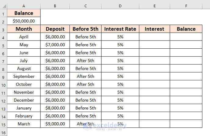
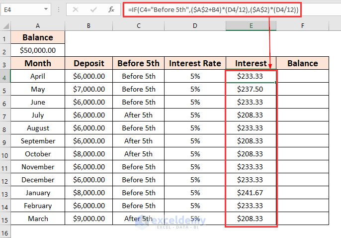
You can use the direct method to calculate the PPF interest easily.
For calculating the PPF interest, we will be using the following dataset. Here, we have the total Balance, Deposits from April to March, and an Interest Rate of 5%.
• For the monthly interest rates use the following formula
=IF(C4=”Before 5th”,($A$2+B4)*(D4/12),($A$2)*(D4/12))
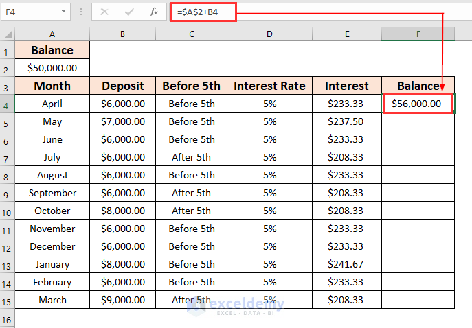
• For the first month of getting the balances, apply the following formula in cell F4.
=$A$2+B4
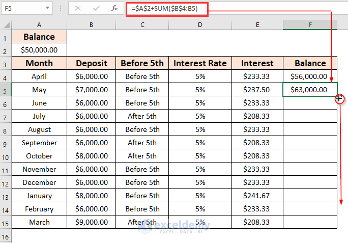
• To get the rest of the balances type the following formula
=$A$2+SUM($B$4:B5)
• Drag down the Fill Handle tool.
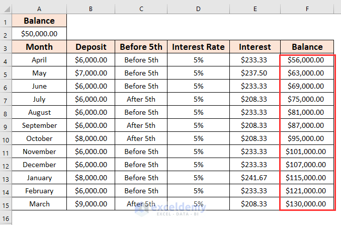
The final output will look like the following figure.
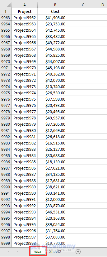
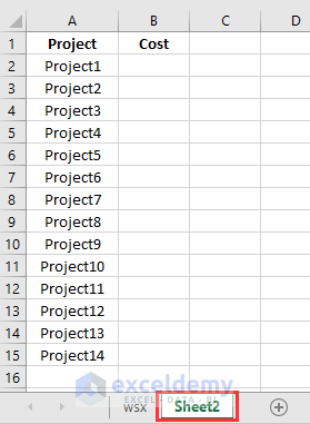
Hi MRBRAT2U,
Thanks for reaching us. You can use the following code to execute your desired operation.
According to your requirement, I have created a source worksheet wsx containing a list of projects with their costs up to 9999 rows.
For the results, we have enlisted some project names in the Sheet2 column and after running the code we will extract the cost values in the Cost column.
• Type the following code in your created module.
• Press F5.
Afterward, you will have the cost values extracted in the Cost column.
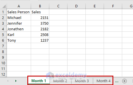
Hi Jeff Blackwell,

Thanks for reaching us. You can use the following code with some adjustments to split a worksheet based on column into some worksheets of the same workbook.
Here, we will split the following worksheet based on the Month column and so the worksheet will be split into 3 different sheets – January, February, March.
• Use the following code. Adjust the starting row number in nRow = 2, the column indicating letter in (the base column on which you will split the worksheet) objWorksheet.Range(“C” & nRow).
• Press F5.
Then, you will have 3 sheets- January, February, March.
Hello Milad,
Thanks for your compliment.
Hi Laurene,
Thanks for staying with us. If the net income cash flows reduced, or 0 or negative, whatever it is. The value of the argument finance rate doesn’t depend on it. You must give the rate as input which is paid by you for cash flows. When you select the payment and incomes at specified intervals as the Values argument, the finance rate as the rate paid by you for your income, and finally the reinvestment rate, the MIRR function will calculate the rate by automatically adjusting the values.
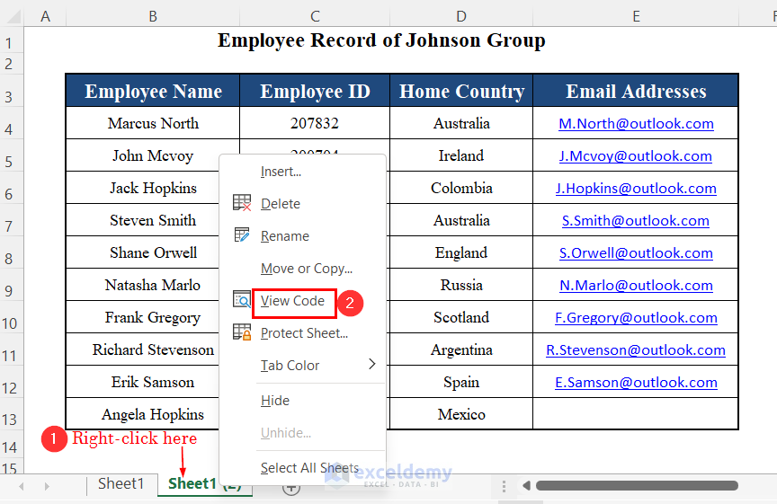
Hi Raymond,
Thanks for your question. I think you can do your task easily by following the code below.
• Right-click on the sheet name containing your dataset and then select the View Code option.
• Type the following code in the opened window and make sure to adjust the number of Target.Column = 5 according to the column number of the emails.
• After saving the code, return to your worksheet.
• Type a random email with @gmail.com
• Press ENTER.
In this way, the email will be automatically changed from gmail to outlook.
Hello Jorge.F,
Thank you so much for your suggestion. I think you might want the following code incorporating your suggested lines. Moreover, I tried to select the range through an input box which may help you select the range.
Hello Julie,
You can try out the following code. I think it will work for you. Just make sure to change the number in Target.Column = 3 according to your column number of data validation.
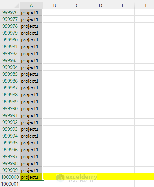
Hi Milad,
Thanks for your question.
According to your requirement, I have created a random dataset containing 1M records within 1M rows of a dataset in Excel. Using a VBA code, I will split it into 10 different worksheets each containing 100,000 rows.
• Type the following VBA code. Here, instead of using the InputBox method, we are directly declaring the total range and the split number in the code which will expediate running the code.
• Press F5.
In this way, we have created 10 different sheets each with 100000 records.
Hi Alex,
Here, I have shown the procedure of creating a waterfall chart for positive increments only. However, you can follow the article of this link- https://www.exceldemy.com/excel-waterfall-chart-with-negative-values/ – to create a chart with negative increment values.
Hi Tushar Chauhan,
kindly let me know which code is causing this problem.
Hello Tushar Chauhan,
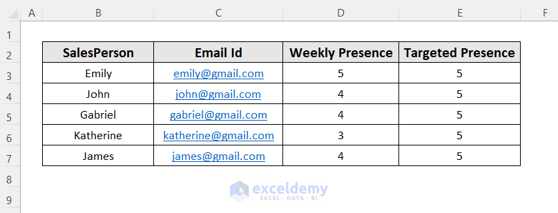
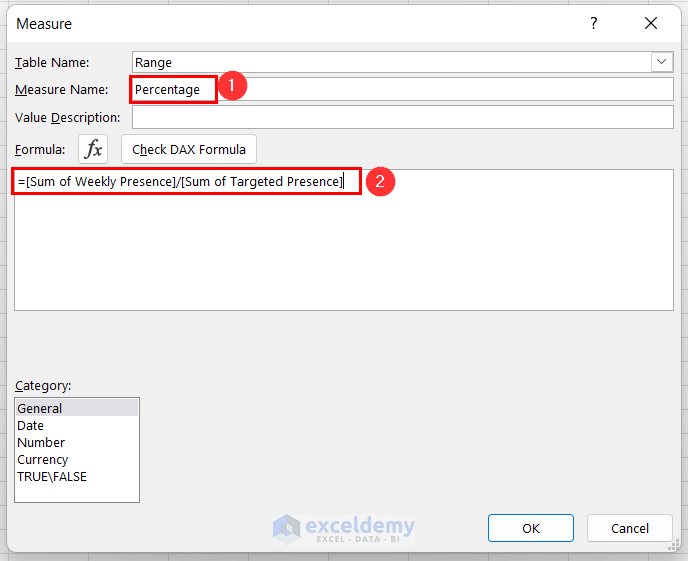
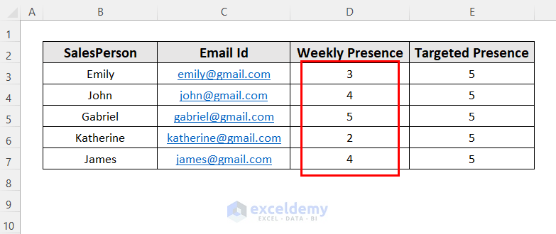
Thanks for reaching us. According to your stated scenario, I have created the following dataset for some imaginary employees. Using their weekly presence and targeted presence we will calculate their weekly percentages here.
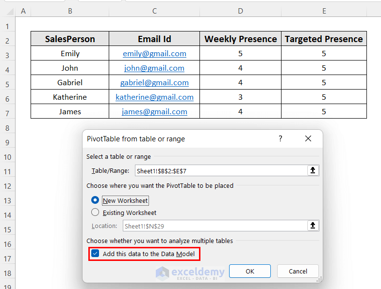
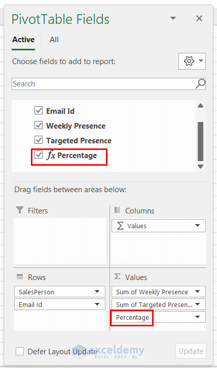
In the process of creating PivotTable, make sure to check the Add this data to the Data Model option.
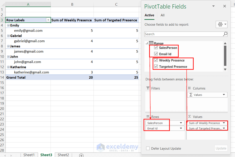
• Drag down the SalesPerson and Email Id fields to the Rows area and Weekly Presence and Targeted Presence fields to the Values area.
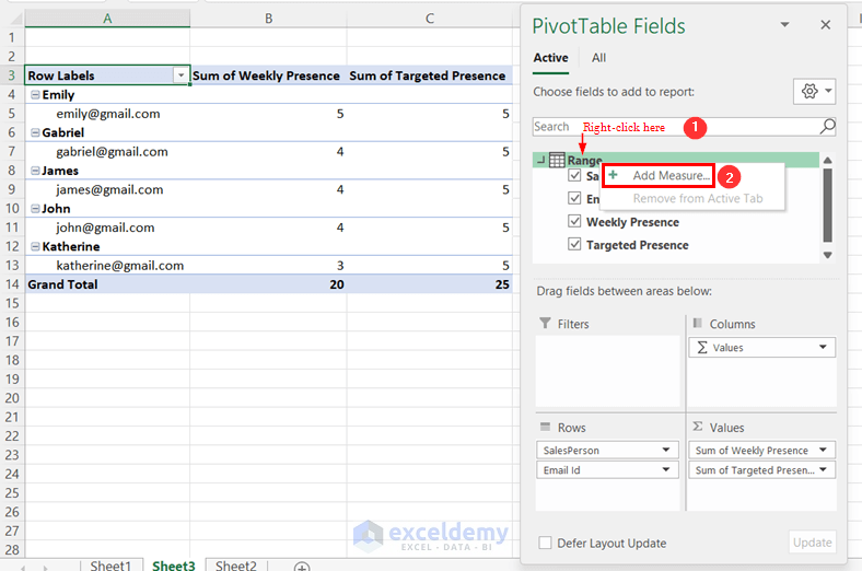
• To add a new measure for calculating percentages right-click on the table name Range and select the Add Measure option.
• In the Measure dialog box, enter Percentage as Measure Name and use the following formula in the Formula box
=[Sum of Weekly Presence]/[Sum of Targeted Presence]
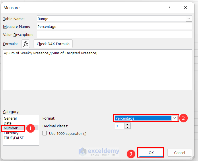
• Choose Number as Category and then select the Percentage option.
• Press OK.
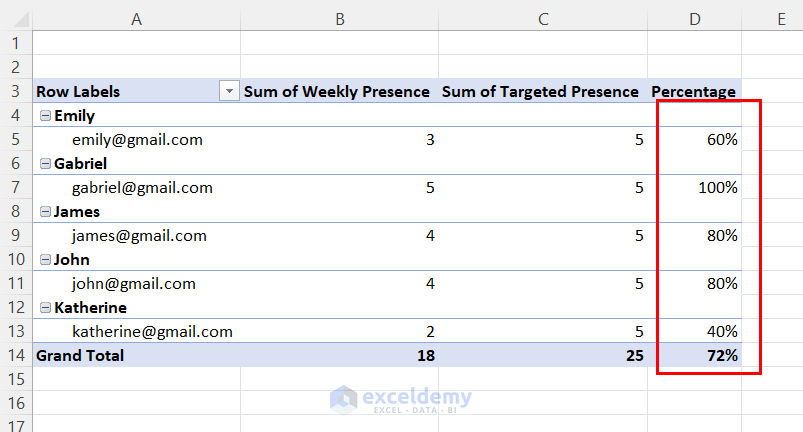
• Drag down the newly created Percentage measure to the Values area.
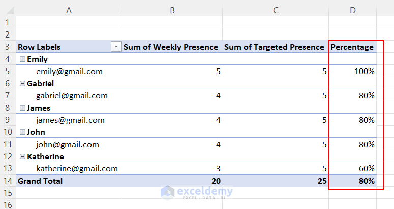
Afterward, you will get the Percentage column in your PivotTable.
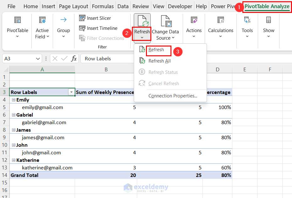
Now, if you change any data of your main dataset then the values of the PivotTable will be updated also.
For instance, we have changed the values of the Weekly Presence column in the main dataset.
• Now go to the sheet with PivotTable and then go to the PivotTable Analyze tab >> Refresh group >> Refresh option.
After that, the percentages will be updated also.
To send these percentages to individual employees automatically using VBA script you can follow this article https://www.exceldemy.com/send-bulk-email-from-outlook-using-excel/
After going through this article, you will notice different ways of doing this task.
Hi Kala,
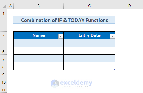
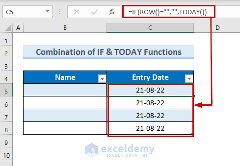
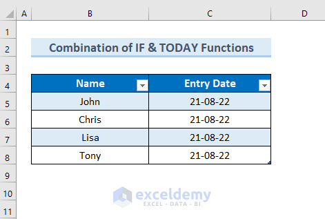
Thanks for your question. According to your comment, you want to work with a table that’s why I have created the following table.
You can use the following formula
=IF(ROW()=””,””,TODAY())
Here, ROW() will return the corresponding row number for a row; like for Row 5, it will give the value 5, for Row 6 you will have 6.
Then, you can insert the names in the Name column.
Hi Jeff V,
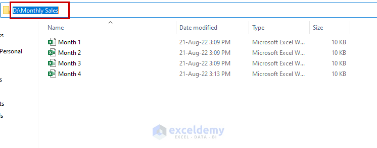
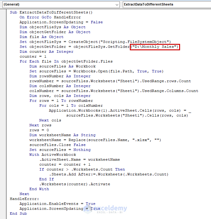
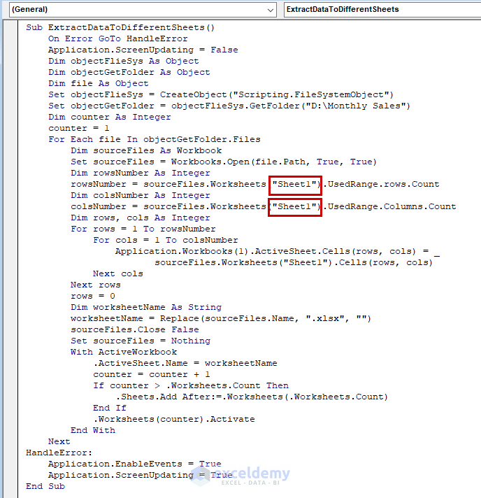
Thanks for reaching us. You have informed us here that the aforementioned code is not giving your expected out. But in my case, I am getting the correct outputs by extracting data from different workbooks into one. I think yours will also work fine if you notice the following matters.
• Firstly, copy the exact path name where your desired files are saved.
• Put down the correct sheet name of your saved workbooks in the following indicated areas.
After modifying all of these factors, run your final code.
Sub ExtractDataToDifferentSheets()
On Error GoTo HandleError
Application.ScreenUpdating = False
Dim objectFlieSys As Object
Dim objectGetFolder As Object
Dim file As Object
Set objectFlieSys = CreateObject(“Scripting.FileSystemObject”)
Set objectGetFolder = objectFlieSys.GetFolder(“D:\Monthly Sales”)
Dim counter As Integer
counter = 1
For Each file In objectGetFolder.Files
Dim sourceFiles As Workbook
Set sourceFiles = Workbooks.Open(file.Path, True, True)
Dim rowsNumber As Integer
rowsNumber = sourceFiles.Worksheets(“Sheet1”).UsedRange.rows.Count
Dim colsNumber As Integer
colsNumber = sourceFiles.Worksheets(“Sheet1”).UsedRange.Columns.Count
Dim rows, cols As Integer
For rows = 1 To rowsNumber
For cols = 1 To colsNumber
Application.Workbooks(1).ActiveSheet.Cells(rows, cols) = _
sourceFiles.Worksheets(“Sheet1”).Cells(rows, cols)
Next cols
Next rows
rows = 0
Dim worksheetName As String
worksheetName = Replace(sourceFiles.Name, “.xlsx”, “”)
sourceFiles.Close False
Set sourceFiles = Nothing
With ActiveWorkbook
.ActiveSheet.Name = worksheetName
counter = counter + 1
If counter > .Worksheets.Count Then
.Sheets.Add After:=.Worksheets(.Worksheets.Count)
End If
.Worksheets(counter).Activate
End With
Next
HandleError:
Application.EnableEvents = True
Application.ScreenUpdating = True
End Sub
Finally, you will get the following sheets in a single workbook.
Hi Andy,
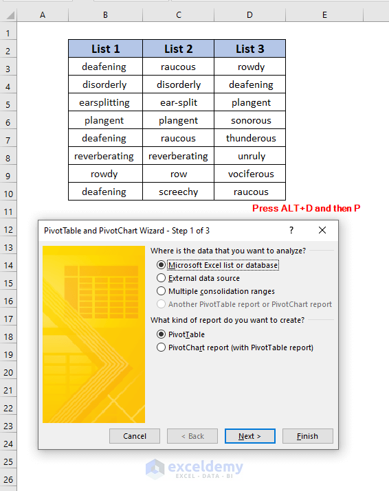
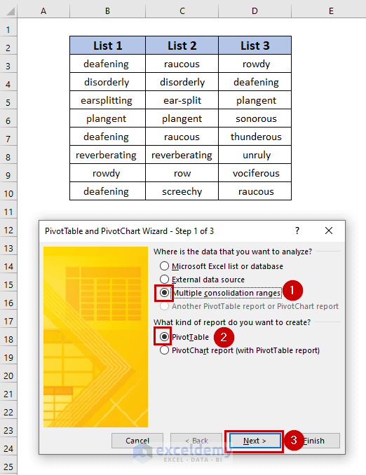
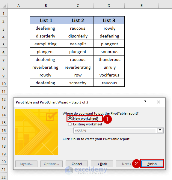
Thanks for your query. Unfortunately, using the UNIQUE function you cannot do your desired job directly. So, I have come up with an easy alternative way.
Here, I have created the following dataset using your example. Using the PivotTable feature of Excel, I will convert the following three columns into a single column with unique values only.
• Press ALT+D and then P immediately to open up the PivotTable and PivotChart Wizard.
• In Step 1 of this wizard click on the options; Multiple consolidation ranges, PivotTable.
• Click on Next.
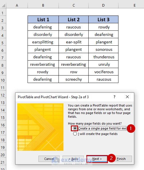
• In Step 2a of this wizard click on the Create a single page field for me option.
• Click on Next.
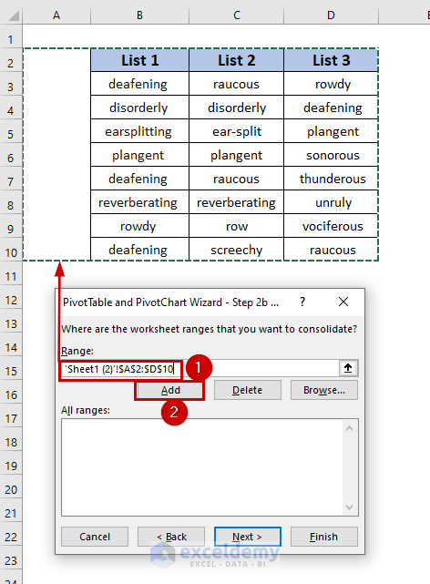
• Now, select the range of the words including a blank column prior to this range in the Range box.
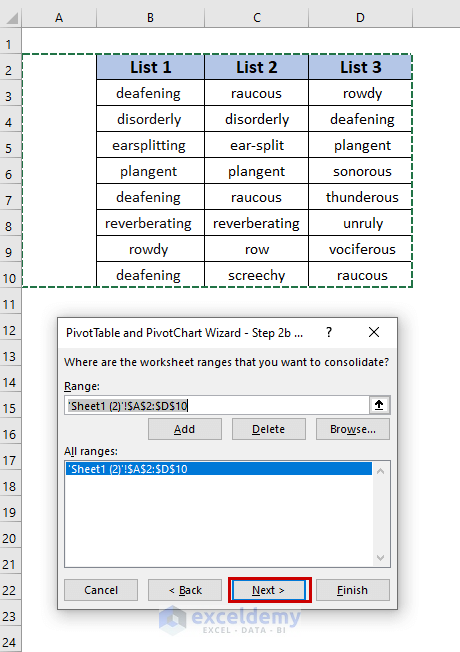
• Select Add to enter the formula of the Range box to the All ranges box.
Afterward, the formula will be entered into the All ranges box, and finally, click on Next.
• In Step 3 of this wizard click on the New worksheet option.
• Click on Finish.
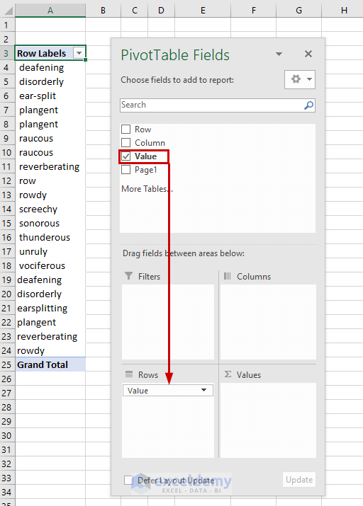
• Now, drag down the Value to the Rows area.
Finally, all of the unique words will be listed in a single column.
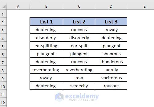
Hello Jen,
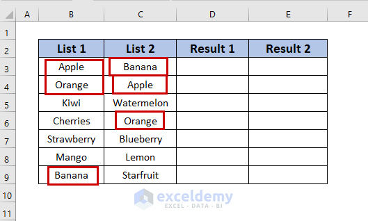
Thanks for your question. I think there is no direct way to fulfill your requirement using the UNIQUE function. But you can use a combination of some functions to get the unique values after comparing different columns.
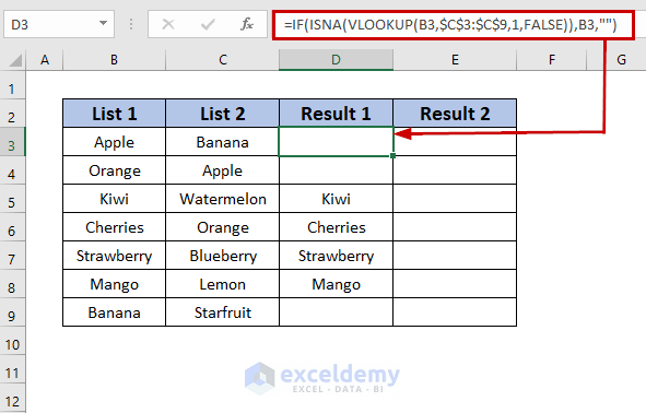
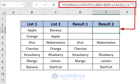
So, I have created the following dataset where I have some names of fruits in the two columns, List 1 and List 2. Here, we have some same fruits names in these two columns, and using the formula we will extract the unique values of these columns in the columns; Result 1, and Result 2.
For extracting the unique values of List 1, we will use the following formula in Result 1.
=IF(ISNA(VLOOKUP(B3,$C$3:$C$9,1,FALSE)),B3,””)
After comparing the unique values of List 2 with the values of List 1 we will use the following formula in the Result 2 column.
=IF(ISNA(VLOOKUP(C3,$B$3:$B$9,1,FALSE)),C3,””)
Hello Dan,
Thank you so much for your appreciation. Hope you will be benefitted more by staying with our Exceldemy site.
Hi David, I think maybe you have forgotten to change the name of the worksheet from another to practice while working with the practice worksheet. So, you can try out the following code to work with the practice sheet.
Sub selectrange1()
Dim LR As Long
Dim x1 As Range, y1 As Range
With ThisWorkbook.Worksheets(“practice”)
LR = Cells(Rows.Count, “B”).End(xlUp).Row
Application.ScreenUpdating = False
For Each x1 In .Range(“B1:B” & LR)
If x1.Text = “Apple” Then
If y1 Is Nothing Then
Set y1 = .Range(“C” & x1.Row).Resize(, 2)
Else
Set y1 = Union(y1, .Range(“C” & x1.Row).Resize(, 2))
End If
End If
Next x1
Application.ScreenUpdating = True
End With
If Not y1 Is Nothing Then y1.Select
End Sub
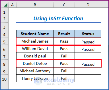
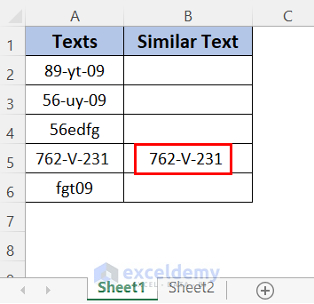
Hello Chandrakant, regarding your problem I have created the following two datasets where in both sheets I have your predefined text 762-V-231. After comparing the range of texts from Sheet1 with Sheet2 I will have the matched texts besides the Existing column.
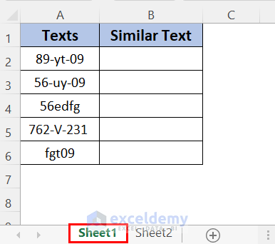
In Sheet1 I have a range of texts and after the comparison, I will have matched texts in the Similar Text column.
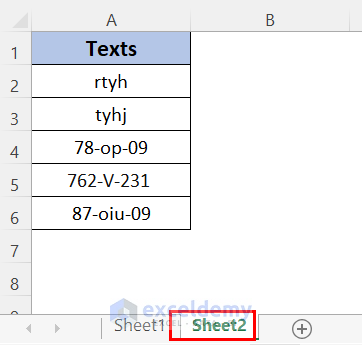
The comparison will be done with Sheet2
To do this comparison you can use the following code
Sub find_text()
Dim source_txt As Range, find_txt As Range
For Each source_txt In Sheets(“Sheet1”).Range(“A2:A6”)
For Each find_txt In Sheets(“Sheet2”).Range(“A2:A6”)
If InStr(1, source_txt, find_txt, vbTextCompare) > 0 Then
source_txt.Offset(0, 1) = find_txt
Exit For
End If
Next
Next
Set source_txt = Nothing
Set find_txt = Nothing
End Sub
After pressing F5, you will have the following result
Hello EXCELLEARNER, Thank you so much for your compliment. Hope you will stay with our site Exceldemy always.
Hello Gabrielle, after going through your problem, I have understood it like this that you want to highlight those dates which are greater than 30 days (or January month) or 60 days (or February month), or 90 days (or March month) and the corresponding specific cells are blank for these dates. If the specific cells are not blank, then the coloring should be avoided. After understanding this scenario, I have created the following dataset like your sample to illustrate the process.
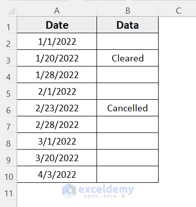
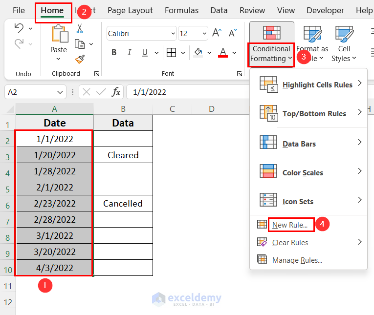
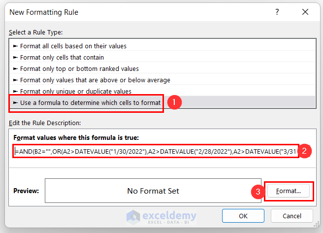
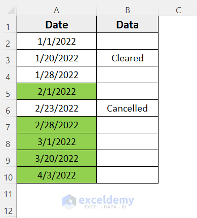
• Firstly, select the dates, and then go to the Home tab >> Conditional Formatting dropdown >> New Rule option.
• In the opening dialog box, choose the indicated option and then type the following formula in the box
=AND(B2=””,OR(A2>DATEVALUE(“1/30/2022”),A2>DATEVALUE(“2/28/2022”),A2>DATEVALUE(“3/31/2022”)))
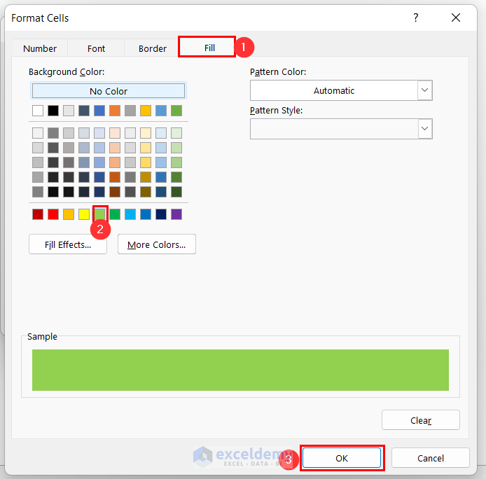
• Click on Format
• In the Format Cells dialog box go to the Fill tab >> select your desired color >> press OK.
Then, the following result will appear.
Hello Richard,
Thanks for your question. The maximum number of sheets in a workbook is 255. So, if you have values for more than 255 rows in a sheet on the basis of which you will create multiple sheets then you may face a problem.
Hello Muizz Shaikh,
Thanks for your question. The maximum number of entries should be within the limit of the maximum row numbers of Excel which is 1,048,576. So, you can merge the files as long as the entries of the combined file support this limit.
Hi Jose A. Valiente, thanks for your valuable suggestion. Actually, the third method is quite different from the first 2 methods as this method determines the P value for the correlation of the two sets of values using a correlation factor.