How to Select Range Based on Cell Value VBA (7 Ways)

If you are looking for some of the easiest ways to select a range based on cell value using VBA, then you are in the right place. You can select a range of cells for different purposes based on another cell value or the same cell value easily by following this article.

Let’s get started with the article.

Download Workbook

7 Ways to Select Range Based On Cell Value VBA

Here, I have the following data table of a company to demonstrate the ways of selecting range based on cell value VBA.

For this purpose, I have used Microsoft Excel 365 version, you can use any other versions according to your convenience.

Method-1: Selecting Range Based On Another Cell Value

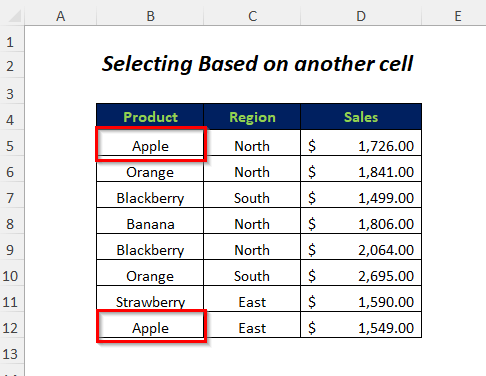
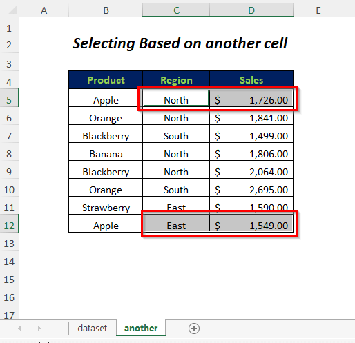
Here, we will select the cell range in the Region and Sales column based on the string Apple in the Product column. To do this follow this method.

Step-01:
➤Go to Developer Tab>>Visual Basic Option

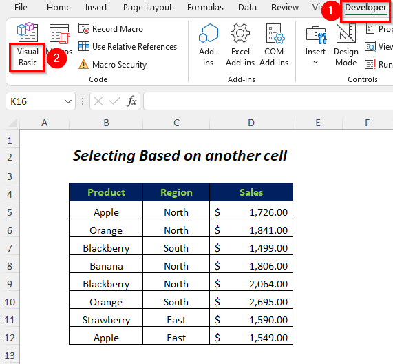
Then, the Visual Basic Editor will open up.
➤Go to Insert Tab>> Module Option

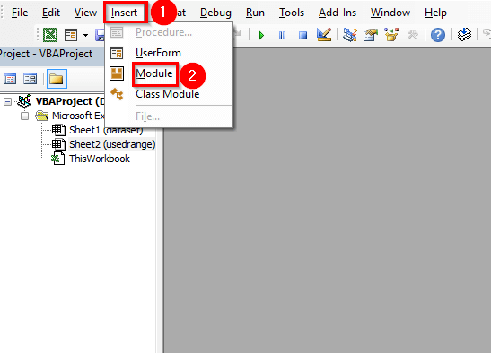
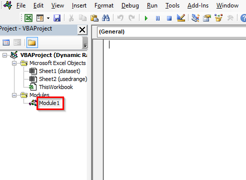
After that, a Module will be created.

Step-02:
➤Write the following code

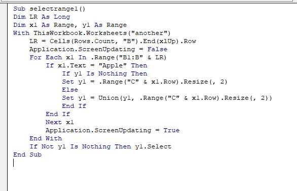
Sub selectrange1()

Dim LR As Long

Dim x1 As Range, y1 As Range

With ThisWorkbook.Worksheets("another")

    LR = Cells(Rows.Count, "B").End(xlUp).Row

    Application.ScreenUpdating = False

    For Each x1 In .Range("B1:B" & LR)

        If x1.Text = "Apple" Then

            If y1 Is Nothing Then

            Set y1 = .Range("C" & x1.Row).Resize(, 2)

            Else

            Set y1 = Union(y1, .Range("C" & x1.Row).Resize(, 2))

            End If

        End If

        Next x1

        Application.ScreenUpdating = True

    End With

    If Not y1 Is Nothing Then y1.Select

End Sub

At first, we declared LR, and x1 and y1 as Long and Range respectively.

Here, “another” is the sheet name, and the WITH statement lets you specify an object or user-defined type once for an entire series of statements.

LR will give you the last row of your data table and FOR loop is used for performing the actions in the range of Column B.

We have used two IF loops, one is for checking the string “Apple” in Column B and the other is for storing the range between Column C and Column D corresponding to the cells having “Apple” in a variable y1.

Here, Range(“C” & x1.Row).Resize(, 2) indicates to selecting two columns from Column C and Union will return the union of multiple ranges corresponding to the cell value “Apple” and finally the ranges will be selected.

➤Press F5

Result:
In this way, you will select the range of cells in the Region and Sales column corresponding to the cell value Apple in the Product column.

Read more: VBA for Each Cell in Range in Excel

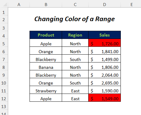
Method-2: Changing Color of a Cell Range Based On Another Cell Value

If you want to change the color of the range of cells in the Sales column based on the cell value Apple in the Product column, then follow this method.

Step-01:
➤Follow Step-01 of Method-1
➤Type the following code

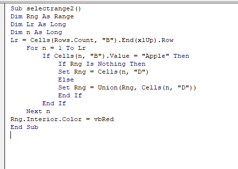
Sub selectrange2()

Dim Rng As Range

Dim Lr As Long

Dim n As Long

Lr = Cells(Rows.Count, "B").End(xlUp).Row

    For n = 1 To Lr

        If Cells(n, "B").Value = "Apple" Then

            If Rng Is Nothing Then

            Set Rng = Cells(n, "D")

            Else

            Set Rng = Union(Rng, Cells(n, "D"))

            End If

        End If

    Next n

Rng.Interior.Color = vbRed

End Sub

At first, we declared Lr and n, and Rng as Long and Range respectively.
Lr will give you the last row of your data table and the FOR loop is used for performing the actions for rows from 1 To Lr.

We have used two IF loops, one is for checking the string “Apple” in Column B for rows 1 To Lr and the other is for storing the range of cells in Column D corresponding to the cells having “Apple” in a variable Rng. Here, Union will return the union of multiple ranges corresponding to the cell value “Apple” and finally the ranges will be colored by red.

➤Press F5

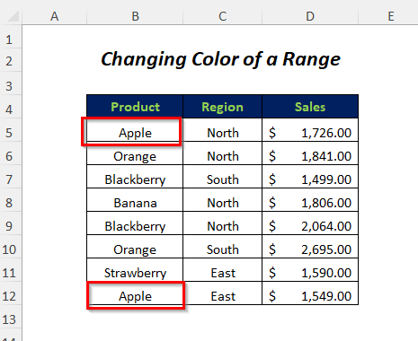
Result:
After that, you will change the color of the range of cells in the Sales column corresponding to the cell value Apple in the Product column.

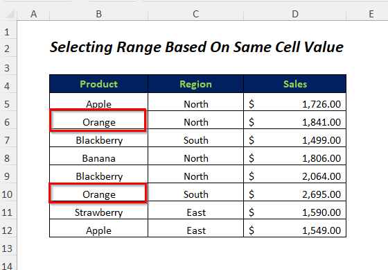
Method-3: Selecting Range Based On Same Cell Value

If you want to select the range of cells in the Product column based on the string Orange in this column, then follow this method.

Step-01:
➤Follow Step-01 of Method-1
➤Type the following code

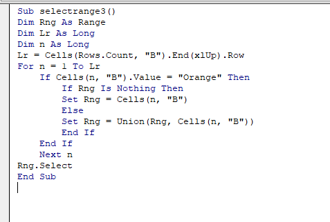
Sub selectrange3()

Dim Rng As Range

Dim Lr As Long

Dim n As Long

Lr = Cells(Rows.Count, "B").End(xlUp).Row

For n = 1 To Lr

    If Cells(n, "B").Value = "Orange" Then

        If Rng Is Nothing Then

        Set Rng = Cells(n, "B")

        Else

        Set Rng = Union(Rng, Cells(n, "B"))

        End If

    End If

    Next n

Rng.Select

End Sub

At first, we declared Lr, n, and Rng as Long and Range respectively.
Lr will give you the last row of your data table and the FOR loop is used for performing the actions for rows from 1 To Lr.

We have used two IF loops, one is for checking the string “Orange” in Column B for rows 1 To Lr and the other is for storing the range of cells in Column B corresponding to the cells having “Orange” in a variable Rng. Here, Union will return the union of multiple ranges corresponding to the cell value “Orange” and finally the ranges will be selected.

➤Press F5

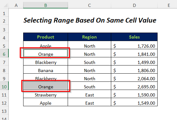
Result:
Afterward, you will select the range of cells in the Product column for the cell value Orange in this column.

Read more: Loop through a Range for Each Cell with Excel VBA

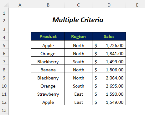
Method-4: Selecting Range Based On Multiple Criteria

If you want to select the cells in the Sales column which have values of more than $1500.00 and less than $2000.00. For selecting cells based on these multiple criteria you can follow this method.

Step-01:
➤Follow Step-01 of Method-1
➤Type the following code

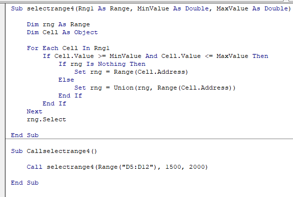
Sub selectrange4(Rng1 As Range, MinValue As Double, MaxValue As Double)

    Dim rng As Range

    Dim Cell As Object

    For Each Cell In Rng1

        If Cell.Value >= MinValue And Cell.Value <= MaxValue Then

            If rng Is Nothing Then

                Set rng = Range(Cell.Address)

            Else

                Set rng = Union(rng, Range(Cell.Address))

            End If

        End If

    Next

    rng.select

End Sub

Sub Callselectrange4()

     Call selectrange4(Range("D5:D12"), 1500, 2000)

End Sub

At first, we declared Rng1, rng, Minvalue, Maxvalue and Cell as Range, Double, and Object respectively.

Here, we used two Sub procedures, the one Callselectrange4() is for calling the other Sub procedure selectrange4 and giving the value of the variables Rng1 as Range(“D5:D12”), Minvalue as 1500, and Maxvalue as 2000 respectively.

Here, one FOR loop and two IF loops have been used in the selectrange4 Sub procedure.

➤Press F5

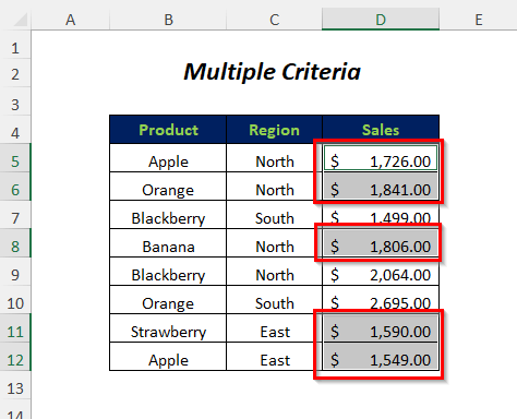
Result:
Then, you will select the range of cells in the Sales column for the cells which have values of more than $1500.00 and less than $2000.00.

Similar Readings:

• VBA to Set Range in Excel (7 Examples)
• How to Use the Range Object of VBA in Excel (5 Properties)
• Use VBA Range Offset (11 Ways)
• VBA to Use Range Based on Column Number in Excel (4 Methods)

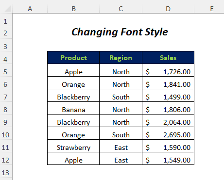
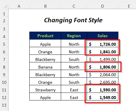
Method-5: Changing Font Style of a Range Based On Multiple Criteria

If you want to bold the fonts of the cells in the Sales column which have values of more than $1500.00 and less than $2000.00. For doing this based on these multiple criteria you can follow this method.

Step-01:
➤Follow Step-01 of Method-1
➤Type the following code

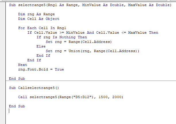
Sub selectrange5(Rng1 As Range, MinValue As Double, MaxValue As Double)

    Dim rng As Range

    Dim Cell As Object

    For Each Cell In Rng1

        If Cell.Value >= MinValue And Cell.Value <= MaxValue Then

            If rng Is Nothing Then

                Set rng = Range(Cell.Address)

            Else

                Set rng = Union(rng, Range(Cell.Address))

            End If

        End If

    Next

    rng.Font.Bold=True

End Sub

Sub Callselectrange5()

     Call selectrange5(Range("D5:D12"), 1500, 2000)

End Sub

At first, we declared Rng1, rng, Minvalue, Maxvalue, and Cell as Range, Double, and Object respectively.

Here, we used two Sub procedures, the one Callselectrange4() is for calling the other Sub procedure selectrange4 and giving the value of the variables Rng1 as Range(“D5:D12”), Minvalue as 1500, and Maxvalue as 2000 respectively.

Here, one FOR loop and two IF loops have been used in the selectrange4 Sub procedure.

➤Press F5

Result:
In this way, you will be able to bold the fonts of the range of cells in the Sales column for the cells which have values of more than $1500.00 and less than $2000.00.

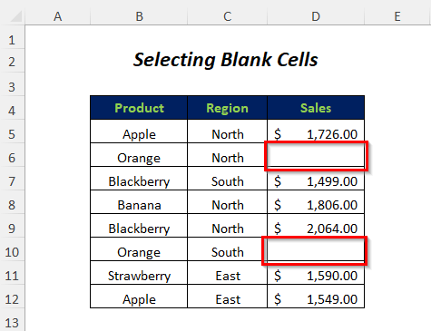
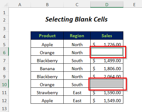
Method-6: Selecting Range Based On Blank Cells

Here, we have some blank cells (I have removed the values for explaining this method) in the Sales column and to select these blank cells we will use the VBA code of this method.

Step-01:
➤Follow Step-01 of Method-1
➤Type the following code

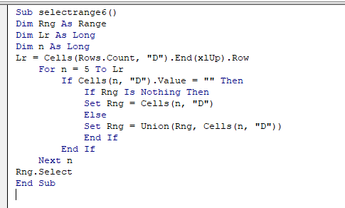
Sub selectrange6()

Dim Rng As Range

Dim Lr As Long

Dim n As Long

Lr = Cells(Rows.Count, "D").End(xlUp).Row

    For n = 5 To Lr

        If Cells(n, "D").Value = "" Then

            If Rng Is Nothing Then

            Set Rng = Cells(n, "D")

            Else

            Set Rng = Union(Rng, Cells(n, "D"))

            End If

        End If

    Next n

Rng.Select

End Sub

At first, we declared Lr, n, and Rng as Long and Range respectively.

Lr will give you the last row of your data table and the FOR loop is used for performing the actions for rows from 5 To Lr. Here, 5 is for the first row of our range.

We have used two IF loops, one is for checking the string “” (Blank) in Column D for rows 1 To Lr and the other is for storing the range of cells in Column D corresponding to the cells having Blank in a variable Rng. Here, Union will return the union of multiple ranges corresponding to the blank cells, and finally, the ranges will be selected.

➤Press F5

Result:
Finally, you will select the blank cells in the column Sales.

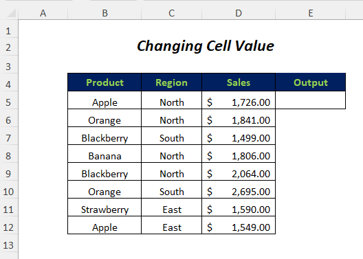
Method-7: Changing Cell Value Based On Selected Cell

Suppose, you want to have the value of the cells in the first cell of the Output column which you select in the Product column. To do this you can follow this method.

Step-01:
➤Follow Step-01 of Method-1
➤Type the following code

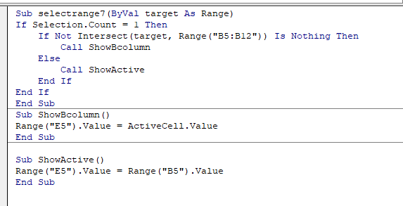
Sub selectrange7(ByVal target As Range)

If Selection.Count = 1 Then

    If Not Intersect(target, Range("B5:B12")) Is Nothing Then

        Call ShowBcolumn

    Else

        Call ShowActive

    End If

End If

End Sub

Sub ShowBcolumn()

Range("E5").Value = ActiveCell.Value

End Sub

Sub ShowActive()

Range("E5").Value = Range("B5").Value

End Sub

Here, we used three Sub procedures, selectrange7 is the main procedure which will call the other two Sub procedures ShowBcolumn() and ShowActive().

Intersect will give the range that is the intersection of two or more ranges and when the selected cell in the dataset is intersected with the range “B5:B12” then it will call ShowBcolumn(). It will return the selected cell’s value in the E5 cell. Otherwise, it will call ShowActive() which will return the value of cell B5.

➤Save the code.
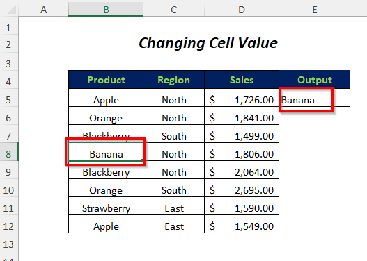
➤Select any cell in the Product column (I have selected the cell containing Banana)
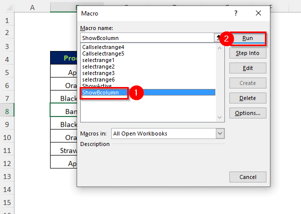
➤Go to Developer Tab>>Macros Option

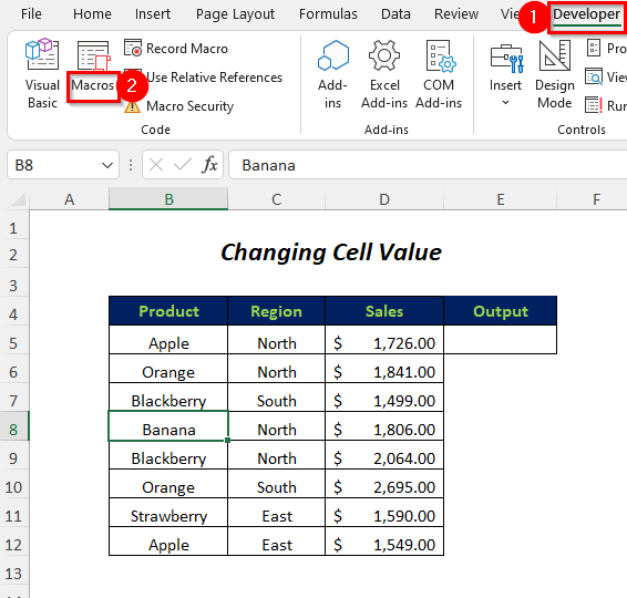
Then Macro Wizard will open up.
➤Select the Macro name ShowBcolumn and then Run.

Result:
Then, you will get the value of the selected cell (Banana) in cell E5.

Practice Section

For doing practice by yourself we have provided a Practice section like below in a sheet named Practice. Please do it by yourself.

Conclusion

In this article, I tried to cover the easiest ways to use VBA effectively while selecting a range based on cell value. Hope you will find it useful. If you have any suggestions or questions, feel free to share them with us.

Further Readings

• Excel VBA Copy Range to Another Sheet (8 Easiest ways)
• How to Count Text in Excel (7 Easy Tricks)
• VBA Range with Variable Row Number in Excel (4 Examples)
• Excel Subscript Out of Range Error in VBA (with 5 Solutions)