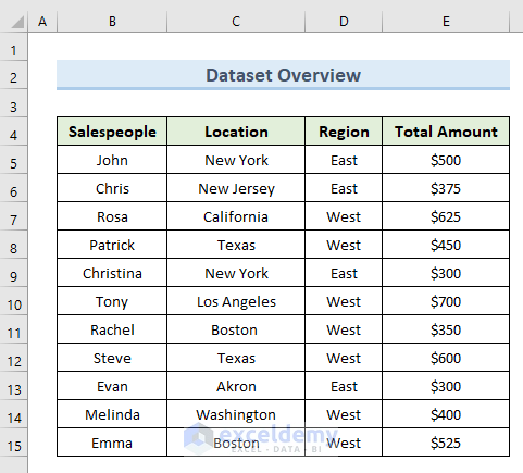
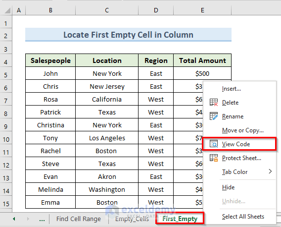
Excel VBA to Select Used Range in Column (8 Examples)

In the following image, we can see the dataset that we will use for all the examples. The dataset contains the names of Salespeople, their Location, Region, and Total Amount of sales. In this dataset, the used range will be considered including the heading (B2:E15).

Example 1 – Select the Used Range in Column with VBA in Excel

We will select all the columns from our dataset.

STEPS:

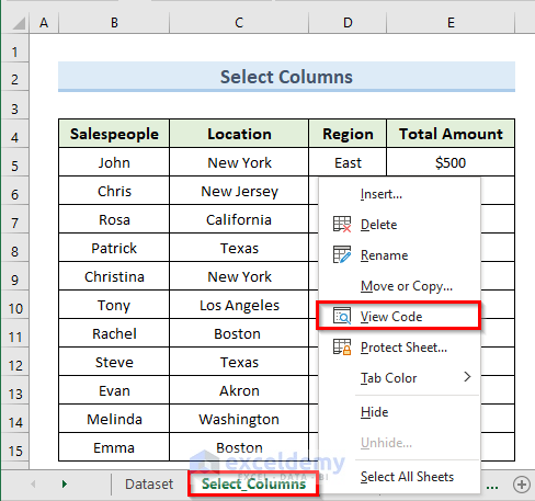
Right-click on the active sheet name ‘Select_Columns’.
Select the option ‘View Code’.

This opens a blank VBA code window for that worksheet.
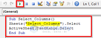
Insert the following code in that code window:

Sub Select_Columns()
Sheets("Select_Columns").Select
ActiveSheet.UsedRange.Select
End Sub

Click on Run or press the F5 key to run the code.

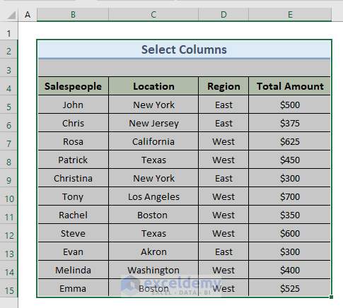
We can see that the used range in columns from our dataset is selected now.

Example 2 – Use VBA to Copy the Entire Used Range

STEPS:

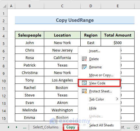
Go to the active worksheet name, ‘Copy’.
Right-click on the name and select the option ‘View Code’.

This will open a blank VBA code window for the current worksheet.
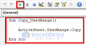
Insert the following code in that code window:

Sub Copy_UsedRange()
ActiveSheet.UsedRange.Copy
End Sub

Click on Run or press the F5 key.

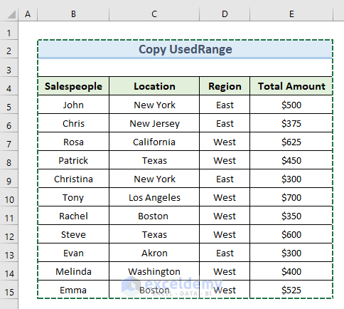
There’s a border around the range indicating that it’s copied to the clipboard.

Example 3 – Count the Number of Columns in the Used Range Using VBA

STEPS:

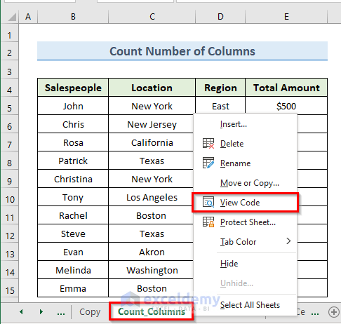
Right-click on the active sheet name and click on the option ‘View Code’.

This opens a blank VBA code window for the active worksheet.
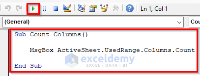
Input the following code in the blank code window:

Sub Count_Columns()
MsgBox ActiveSheet.UsedRange.Columns.Count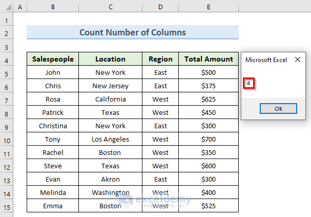
End Sub

Click on Run or press the F5 key to run the code.

We get the result in a message box.

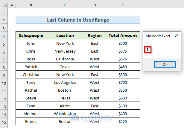
Example 4 – Excel VBA to Get the Number of the Last Column in the Used Range

STEPS:

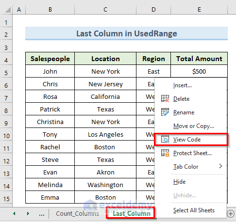
Right-click on the active sheet name ‘Last Column’.
Select the option ‘View Code’.

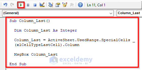
Insert the following code in the code window:

Sub Column_Last()
Dim Column_Last As Integer
Column_Last = ActiveSheet.UsedRange.SpecialCells(xlCellTypeLastCell).Column
MsgBox Column_Last
End Sub

Click on Run or press the F5 key to run the code.

We get our result in a message box. The last column in the used range is the 5th column in the worksheet.

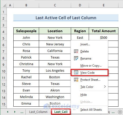
Example 5 – Select the Last Cell of the Last Column from the Used Range with VBA

STEPS:

Right-click on the active sheet name.
Select the option ‘View Code’.

We get a blank VBA code window.
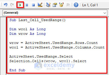
Insert the following code in that code window:

Sub Last_Cell_UsedRange()
Dim wcol As Long
Dim wrow As Long
wrow = ActiveSheet.UsedRange.Rows.Count
wcol = ActiveSheet.UsedRange.Columns.Count
ActiveSheet.UsedRange.Select
Selection.Cells(wrow, wcol).Select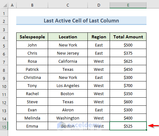
End Sub

Click on Run or press the F5.

We can see the result in the following image. The selected last cell of the last column is cell E15.

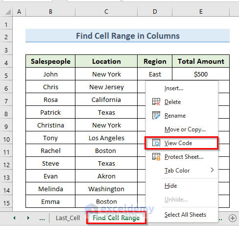
Example 6 – Find the Cell Range of the Selected the Used Range with Excel VBA

STEPS:

Right-click on the active sheet tab name, in the example ‘Find Cell Range’.
Select the option ‘View Code’.

This will open a blank VBA code window.
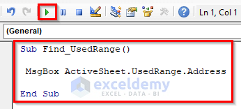
Enter the following code in that code window:

Sub Find_UsedRange()
MsgBox ActiveSheet.UsedRange.Address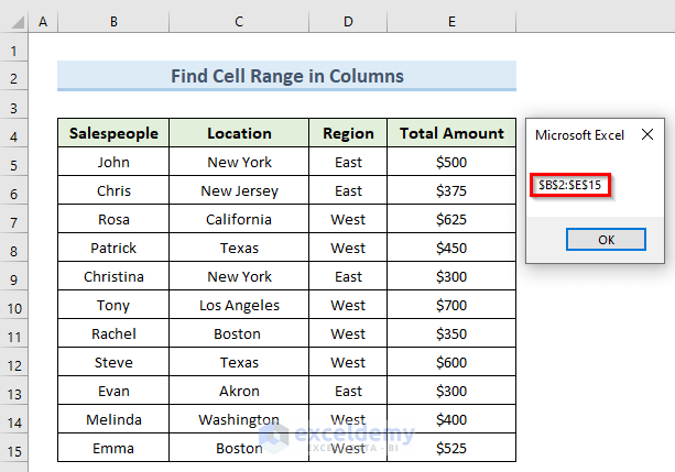
End Sub

Click on Run or press the F5 key.

A message box like the following image shows the result.

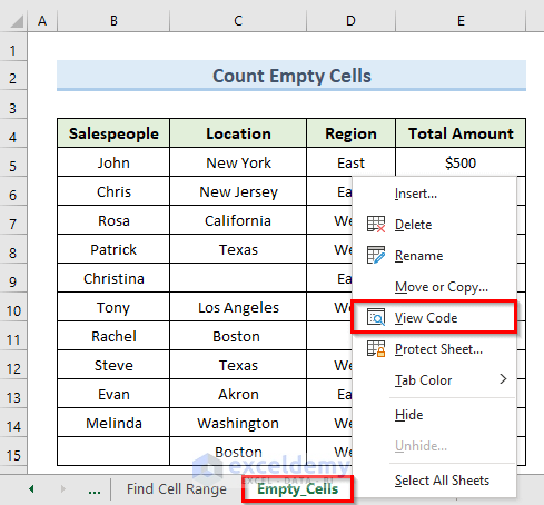
Example 7 – Insert the VBA UsedRange Property to Count Empty Cells

STEPS:

Right-click on the active sheet tab name, ‘Empty_Cells’.
Select the option ‘View Code’.

This opens a blank VBA code window.
Insert the following code in the code window:

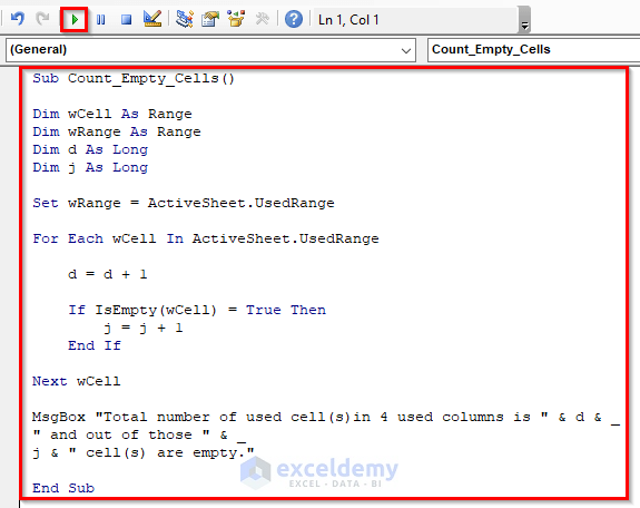
Sub Count_Empty_Cells()
Dim wCell As Range
Dim wRange As Range
Dim d As Long
Dim j As Long
Set wRange = ActiveSheet.UsedRange
For Each wCell In ActiveSheet.UsedRange
d = d + 1
If IsEmpty(wCell) = True Then
j = j + 1
End If
Next wCell
MsgBox "Total number of used cell(s)in 4 used columns is " & d & _
" and out of those " & _
j & " cell(s) are empty."
End Sub

Click on Run or press the F5 key to run the code.

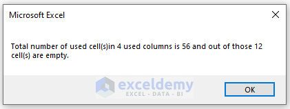
We will get the result in the message box. The message box will display the number of total cells and blank cells in our used range.

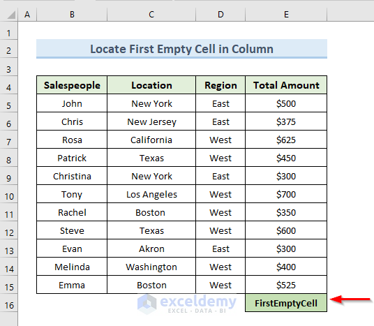
Example 8 – VBA UsedRange to Locate the Next Empty Cell in the Last Column of the Used Range

STEPS:

Right-click on the active sheet tab, named ‘First_Empty’.
Select the option ‘View Code’.

This will open a blank VBA code window.
Insert the following code in the blank VBA code window:

Public Sub First_Empty_Cell()
ActiveSheet.Range("E" & ActiveSheet.Rows.Count) _
.End(xlUp).Offset(1, 0).Value = "FirstEmptyCell"
End Sub

Click on Run or press the F5 key.

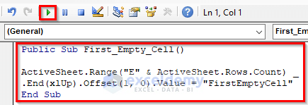
The above code will insert the value ‘FirstEmptyCell’ in cell E16. It is the first empty cell of column E after the used range of the dataset.