Latest Posts From Sanjida Mehrun Guria

In Microsoft Excel, there is no inbuilt function named RegEx. Rather we have to create it manually in the workbook. This function is required to prohibit the ...

In mathematics, calculating combinations of a certain number of characters is a very common practice. In fact, we can count these combinations in Microsoft ...

In our regular life, we often notice numbers with suffix letters such as product code, zip code, account code, insurance numbers, and lots more. But the ...

Sometimes while executing formulas, incorrect values are returned despite the formulas being correct. This may happen as a result of dirty cells and their ...

Microsoft Excel is a powerful tool to create a dynamic database. We can store the data of our device folders or browsers which is called Metadata. In this ...

Depreciation is a very common term in the case of assets. In general, it is the decline of an asset over a certain period of time. There are many methods to ...

Zip codes are defined as the postal code of certain cities or states of a country. It is used as a part of the address. Every country has its database of zip ...

Issue 1 - Unable to Edit Embedded Excel Chart in PowerPoint Select the cell range B4:C14 as we want to create a chart out of these values. Go to ...

Google Forms is a popular tool for creating online surveys and quizzes, which can be used for everything from market research to customer feedback. This ...
Types of Relationships Between Tables in Excel In Excel, we can create three different types of relationships among tables. They are: 1. ...
Counting characters at the beginning of a word using the COUNTIF & LEFT Functions in Excel – 3 Steps
STEP 1 - Create a Dataset Create a dataset. Here, B4:C15. STEP 2 - Enter the Text You Need to Count In F6 (Search), enter B to count the ...
![[Fixed!] Excel VLOOKUP Function Not Calculating Automatically](https://www.exceldemy.com/wp-content/uploads/2022/11/VLOOKUP-Not-Calculating-Automatically-4-1.png?v=1697442071)
In Excel, the VLOOKUP function is a very popular one for fetching data among large datasets. But sometimes we face difficulties when VLOOKUP does not calculate ...
![[Fixed!] Excel Hyperlink Keeps Coming Back (5 Quick Solutions)](https://www.exceldemy.com/wp-content/uploads/2022/11/Excel-Hyperlink-Keeps-Coming-Back-6.png?v=1697442158)
A hyperlink is a form of text that refers to a certain web address with a URL link. Microsoft Excel allows us to auto-hyperlink any text whenever we type it in ...
![[Fixed!] Macros Not Working in Excel (3 Possible Solutions)](https://www.exceldemy.com/wp-content/uploads/2022/11/Macros-Not-Working-in-Excel-3-6.png?v=1697441923)
We prepared a sample dataset here with the First Names, Last Names, and Ages of six people. We want to copy a single cell from the dataset with this ...
Overview of the IMPORTRANGE Function Function Objective The IMPORTRANGE function allows you to retrieve specific ranges of values from an Excel ...
- « Previous Page
- 1
- 2
- 3
- 4
- …
- 7
- Next Page »
See Our Reviews at


Hello Nah,
Thanks for your feedback. As mentioned in the article, you can try any of the methods for your preferred hours. Only the CONVERT function cannot do that because it is built to perform on standard time format. Therefore, please check the attached Excel file where the working day is considered 8 hours/day.
https://www.exceldemy.com/wp-content/uploads/2023/04/Convert-Hours-to-Days.xlsx
Thank you.
Regards,
Sanjida Mehrun Guria
Excel VBA & Content Developer
ExcelDemy
Hello Jon,
Thank you for sharing your query. I have gone through your shared dataset but the values and their required output seem quite unclear in your question. Still, I have tried to solve it. You will find the solution in the Excel file below.
https://www.exceldemy.com/wp-content/uploads/2023/04/Index-match-duplicate-values.xlsx
Please go through it and let us know if it is the solution that you are looking for. Otherwise, feel free to share your Excel file with [email protected] and we will look into this deeply.
Thank you.
Regards,
Sanjida Mehrun Guria
Excel VBA & Content Developer
ExcelDemy
Hello Jake,
Thanks for sharing your query. Please find the attached Excel file with the solution. Let us know for more queries.
https://www.exceldemy.com/wp-content/uploads/2023/04/Calculate-Distance-Between-Two-Cities.xlsx
Thank you.
Regards,
Sanjida Mehrun Guria
Excel VBA & Content Developer
ExcelDemy
Hello Luis,
Thank you for sharing your problem with us. As per your referred formula, I assume it is difficult to insert each product’s price in Column D for alignment. Because you need to have 2 separate datasets comprising Products and their Prices. Only after that, you can align them individually based on each category. For this, go through the following solutions that we described in this article.
Using VLOOKUP Function to Line up Two Sets of Data in Excel
https://www.exceldemy.com/align-two-sets-of-data-in-excel/#1_Using_VLOOKUP_Function_to_Line_up_Two_Sets_of_Data_in_Excel
Use of Consolidate Feature for Summing Up Values within Two Sets of Data in Excel
https://www.exceldemy.com/align-two-sets-of-data-in-excel/#5_Use_of_Consolidate_Feature_for_Summing_Up_Values_within_Two_Sets_of_Data_in_Excel
I hope it will help you. Let us know your feedback.
Thank you.
Regards,
Sanjida Mehrun Guria
Excel VBA & Content Developer
ExcelDemy
Hello Scott,
Thank you for sharing your problem. As per your query, you can simultaneously format specific text in Bold, Italic, Underline and even change Font Size with the following code.
Sub Highlight_a_Single_Specific_Text_Case_Insensitive()Text = InputBox("Enter the Specific Text: ")Color_Code = Int(InputBox("Enter the Color Code: " + vbNewLine + "Enter 3 for Color Red." + vbNewLine + "Enter 5 for Color Blue." + vbNewLine + "Enter 6 for Color Yellow." + vbNewLine + "Enter 10 for Color Green."))For i = 1 To Selection.Rows.CountFor j = 1 To Selection.Columns.CountFor k = 1 To Len(Selection.Cells(i, j))If LCase(Mid(Selection.Cells(i, j), k, Len(Text))) = LCase(Text) ThenSelection.Cells(i, j).Characters(k, Len(Text)).Font.ColorIndex = Color_CodeSelection.Cells(i, j).Characters(k, Len(Text)).Font.Bold = TrueSelection.Cells(i, j).Characters(k, Len(Text)).Font.Italic = TrueSelection.Cells(i, j).Characters(k, Len(Text)).Font.Underline = TrueSelection.Cells(i, j).Characters(k, Len(Text)).Font.Size = 16End IfNext kNext jNext iEnd SubApply this code to the selected cells of your dataset and you will get the desired output.
I hope this solution will help you. Waiting to get your feedback.
Regards,
Guria
ExcelDemy
Hello Nicola,
Thank you for sharing your problem. I assume you are getting difficulties to calculate interest rate as changed twice in a year. In that case, calculate first 6 months’ rate separately with this formula =7.5/12 and later 6 months’ with =8/12. As a result, you will get the values of monthly interests.
I hope this solution will help you. Let us know your feedback.
Regards,
Guria
ExcelDemy
Hello Donald Duck,
Thank you for sharing your wonderful tip to hide the secondary axis in Excel. I hope it will profoundly help our users.
Regards,
Guria
ExcelDemy
Hello Naureen,
Thank you for sharing your problem. I am replying on behalf of ExcelDemy. Assuming the student names are in Column A and the scores are in Column B, insert this formula to get the top 10 scorers with duplicate values.
=INDEX(SORT(A2:B16,2,-1),SEQUENCE(10),1)If you want to get the names in another sheet, then just add the worksheet names in the formula (as shown below) and you will get your required output.
=INDEX(SORT(‘Semester 2’!A2:B16,2,-1),SEQUENCE(10),1)I hope this solution will help you. Otherwise, feel free to share your workbook with [email protected] and we will look into this deeply.
Regards,
Guria
ExcelDemy
Hello ExcelIsAbandonware,
Thank you for sharing this Excel bug issue with the solution. I hope it will profoundly help our users.
Regards,
Guria
ExcelDemy
Hello Arif,
Thank you for sharing your query with us. As per your question, there can be 2 solutions to the problem.
1. If your number is 100000, then convert it to One Lac with this formula where Thousand is kept blank.
=CHOOSE(LEFT(TEXT(H6,"000000000.00"))+1,,"One","Two","Three","Four","Five","Six","Seven","Eight","Nine")
&IF(--LEFT(TEXT(H6,"000000000.00"))=0,,IF(AND(--MID(TEXT(H6,"000000000.00"),2,1)=0,--MID(TEXT(H6,"000000000.00"),3,1)=0)," Lac"," Lac and "))
&CHOOSE(MID(TEXT(H6,"000000000.00"),2,1)+1,,,"Twenty ","Thirty ","Forty ","Fifty ","Sixty ","Seventy ","Eighty ","Ninety ")
&IF(--MID(TEXT(H6,"000000000.00"),2,1)<>1,CHOOSE(MID(TEXT(H6,"000000000.00"),3,1)+1,,"One","Two","Three","Four","Five","Six","Seven","Eight","Nine"),
CHOOSE(MID(TEXT(H6,"000000000.00"),3,1)+1,"Ten","Eleven","Twelve","Thirteen","Fourteen","Fifteen","Sixteen","Seventeen","Eighteen","Nineteen"))
&IF((--LEFT(TEXT(H6,"000000000.00"))+MID(TEXT(H6,"000000000.00"),2,1)+MID(TEXT(H6,"000000000.00"),3,1))=0,,IF(AND((--MID(TEXT(H6,"000000000.00"),4,1)+MID(TEXT(H6,"000000000.00"),5,1)+MID(TEXT(H6,"000000000.00"),6,1)+MID(TEXT(H6,"000000000.00"),7,1))=0,(--MID(TEXT(H6,"000000000.00"),8,1)+RIGHT(TEXT(H6,"000000000.00")))>0)," Crore and "," Crore "))
&CHOOSE(MID(TEXT(H6,"000000000.00"),4,1)+1,,"One","Two","Three","Four","Five","Six","Seven","Eight","Nine")
&IF(--MID(TEXT(H6,"000000000.00"),4,1)=0,,IF(AND(--MID(TEXT(H6,"000000000.00"),5,1)=0,--MID(TEXT(H6,"000000000.00"),6,1)=0)," Lac"," Lac"))
&CHOOSE(MID(TEXT(H6,"000000000.00"),5,1)+1,,," Twenty"," Thirty"," Forty"," Fifty"," Sixty"," Seventy"," Eighty"," Ninety")
&IF(--MID(TEXT(H6,"000000000.00"),5,1)<>1,CHOOSE(MID(TEXT(H6,"000000000.00"),6,1)+1,," One"," Two"," Three"," Four"," Five"," Six"," Seven"," Eight"," Nine"),CHOOSE(MID(TEXT(H6,"000000000.00"),6,1)+1," Ten"," Eleven"," Twelve"," Thirteen"," Fourteen"," Fifteen"," Sixteen"," Seventeen"," Eighteen"," Nineteen"))
&IF((--MID(TEXT(H6,"000000000.00"),4,1)+MID(TEXT(H6,"000000000.00"),5,1)+MID(TEXT(H6,"000000000.00"),6,1))=0,,IF(OR((--MID(TEXT(H6,"000000000.00"),7,1)+MID(TEXT(H6,"000000000.00"),8,1)+MID(TEXT(H6,"000000000.00"),9,1))=0,--MID(TEXT(H6,"000000000.00"),7,1)<>0),"  ","  "))
&CHOOSE(MID(TEXT(H6,"000000000.00"),7,1)+1,,"One","Two","Three","Four","Five","Six","Seven","Eight","Nine")
&IF(--MID(TEXT(H6,"000000000.00"),7,1)=0,,IF(AND(--MID(TEXT(H6,"000000000.00"),8,1)=0,--MID(TEXT(H6,"000000000.00"),9,1)=0)," Hundred "," Hundred and "))&
CHOOSE(MID(TEXT(H6,"000000000.00"),8,1)+1,,,"Twenty ","Thirty ","Forty ","Fifty ","Sixty ","Seventy ","Eighty ","Ninety ")
&IF(--MID(TEXT(H6,"000000000.00"),8,1)<>1,CHOOSE(MID(TEXT(H6,"000000000.00"),9,1)+1,,"One","Two","Three","Four","Five","Six","Seven","Eight","Nine"),CHOOSE(MID(TEXT(H6,"000000000.00"),9,1)+1,"Ten","Eleven","Twelve","Thirteen","Fourteen","Fifteen","Sixteen","Seventeen","Eighteen","Nineteen"))
2. If your number is 123450, convert it into a word with this formula.
=CHOOSE(LEFT(TEXT(H6,"000000000.00"))+1,,"One","Two","Three","Four","Five","Six","Seven","Eight","Nine")
&IF(--LEFT(TEXT(H6,"000000000.00"))=0,,IF(AND(--MID(TEXT(H6,"000000000.00"),2,1)=0,--MID(TEXT(H6,"000000000.00"),3,1)=0)," Lac"," Lac and "))
&CHOOSE(MID(TEXT(H6,"000000000.00"),2,1)+1,,,"Twenty ","Thirty ","Forty ","Fifty ","Sixty ","Seventy ","Eighty ","Ninety ")
&IF(--MID(TEXT(H6,"000000000.00"),2,1)<>1,CHOOSE(MID(TEXT(H6,"000000000.00"),3,1)+1,,"One","Two","Three","Four","Five","Six","Seven","Eight","Nine"),
CHOOSE(MID(TEXT(H6,"000000000.00"),3,1)+1,"Ten","Eleven","Twelve","Thirteen","Fourteen","Fifteen","Sixteen","Seventeen","Eighteen","Nineteen"))
&IF((--LEFT(TEXT(H6,"000000000.00"))+MID(TEXT(H6,"000000000.00"),2,1)+MID(TEXT(H6,"000000000.00"),3,1))=0,,IF(AND((--MID(TEXT(H6,"000000000.00"),4,1)+MID(TEXT(H6,"000000000.00"),5,1)+MID(TEXT(H6,"000000000.00"),6,1)+MID(TEXT(H6,"000000000.00"),7,1))=0,(--MID(TEXT(H6,"000000000.00"),8,1)+RIGHT(TEXT(H6,"000000000.00")))>0)," Crore and "," Crore "))
&CHOOSE(MID(TEXT(H6,"000000000.00"),4,1)+1,,"One","Two","Three","Four","Five","Six","Seven","Eight","Nine")
&IF(--MID(TEXT(H6,"000000000.00"),4,1)=0,,IF(AND(--MID(TEXT(H6,"000000000.00"),5,1)=0,--MID(TEXT(H6,"000000000.00"),6,1)=0)," Lac"," Lac"))
&CHOOSE(MID(TEXT(H6,"000000000.00"),5,1)+1,,," Twenty"," Thirty"," Forty"," Fifty"," Sixty"," Seventy"," Eighty"," Ninety")
&IF(--MID(TEXT(H6,"000000000.00"),5,1)<>1,CHOOSE(MID(TEXT(H6,"000000000.00"),6,1)+1,," One"," Two"," Three"," Four"," Five"," Six"," Seven"," Eight"," Nine"),CHOOSE(MID(TEXT(H6,"000000000.00"),6,1)+1," Ten"," Eleven"," Twelve"," Thirteen"," Fourteen"," Fifteen"," Sixteen"," Seventeen"," Eighteen"," Nineteen"))
&IF((--MID(TEXT(H6,"000000000.00"),4,1)+MID(TEXT(H6,"000000000.00"),5,1)+MID(TEXT(H6,"000000000.00"),6,1))=0,,IF(OR((--MID(TEXT(H6,"000000000.00"),7,1)+MID(TEXT(H6,"000000000.00"),8,1)+MID(TEXT(H6,"000000000.00"),9,1))=0,--MID(TEXT(H6,"000000000.00"),7,1)<>0),"  ","  "))
&CHOOSE(MID(TEXT(H6,"000000000.00"),7,1)+1,,"One","Two","Three","Four","Five","Six","Seven","Eight","Nine")
&IF(--MID(TEXT(H6,"000000000.00"),7,1)=0,,IF(AND(--MID(TEXT(H6,"000000000.00"),8,1)=0,--MID(TEXT(H6,"000000000.00"),9,1)=0)," Hundred "," Hundred and "))&
CHOOSE(MID(TEXT(H6,"000000000.00"),8,1)+1,,,"Twenty ","Thirty ","Forty ","Fifty ","Sixty ","Seventy ","Eighty ","Ninety ")
&IF(--MID(TEXT(H6,"000000000.00"),8,1)<>1,CHOOSE(MID(TEXT(H6,"000000000.00"),9,1)+1,,"One","Two","Three","Four","Five","Six","Seven","Eight","Nine"),CHOOSE(MID(TEXT(H6,"000000000.00"),9,1)+1,"Ten","Eleven","Twelve","Thirteen","Fourteen","Fifteen","Sixteen","Seventeen","Eighteen","Nineteen"))
I hope this solution will help you. Let us know your feedback.
Regards,
Guria
ExcelDemy
Hello Felix,
Thank you for sharing your query. Unfortunately, you cannot expressly create a hyperlink for a single word in a text string under a cell. By default, Excel creates a hyperlink for the whole cell. But you can change the cell appearance to show the hyperlink only to a single word. For this, do the following tasks.
• First, create a hyperlink for the whole text following any methods from this article.
• Then, select the words that you don’t want to be shown as hyperlinks.
• Now, remove Underline from the selected texts from the Home tab or by pressing Ctrl + U on your keyboard.
• Along with it, change the Font Color to Automatic.
• Finally, the output will look like this.
I hope this will help you with your problem. Eagerly waiting for your feedback.
Thank you.
Regards,
Guria
ExcelDemy
Hello Edmund Goh,
Thank you for sharing your problem with us. I assume you have properly gone through the steps to separate numbers with the Text to Columns feature. The reason that any changes are not updating is because the Text to Columns feature is static and it will not take any changes from the source cell. Yes, this is a limitation of this feature. You will also face the same if you apply the Flash Fill feature. In this case, I will suggest you to apply any other methods from this article except Method 4 and 5. Then you will be able to get changes on the separated numbers from the text.
Let us know if it helps you.
Thank you.
Regards,
Guria
ExcelDemy.
Hello Theva,
Glad that you shared your query. As per your given example, if you want to simplify the first letter of each word along with numbers, apply this simple VBA code.
Function ExtractFirstLetters(rng As Range) As StringDim arryDim X As Longarry = VBA.Split(rng, " ")If IsArray(arry) ThenFor X = LBound(arry) To UBound(arry)ExtractFirstLetters = ExtractFirstLetters & Left(arry(X), 1)Next XElseExtractFirstLetters = Left(arry, 1)End IfEnd FunctionNote that, if the words in your dataset are separated by Hyphens (–) then insert this line in the code
arry = VBA.Split(rng, "-")Instead of this,
arry = VBA.Split(rng, " ")I hope this will solve your problem. Let us know your feedback.
Regards,
Guria
ExcelDemy.
Hello Mike,
Thanks for sharing your problem. It seems fine for me when I tried to save the excel file shared in this article. The timestamp does not change in my case. Therefore, I will suggest you go through the steps carefully, no matter which method you prefer. Also, please check if the Enable iterative calculation option in File > Options > Formulas section is turned on. If it still changes then try the VBA code shared in this article.
https://www.exceldemy.com/timestamp-in-excel-when-cell-changes/#2_Apply_VBA_Code_to_Insert_Timestamp_in_Excel_When_Cell_Changes
Let us know if you can solve the issue. Otherwise, please send us the excel file that you are working on at this address [email protected].
Regards,
Guria
ExcelDemy.
Hello Violet,
Thanks for sharing your query. Yes, the PMT does include tax or insurance. Therefore, you will provide $1308 as the PMT in your spreadsheet.
Let us know if you have more queries.
Regards,
Guria
ExcelDemy.
Hello Tony Woods,
Thank you for sharing your query. I have tried to change values in the Level column and the timestamp changes according to the custom date format you shared. So it seems there is nothing wrong with your preferred custom format or the method that we described in the article. Therefore, I have come to the following solutions to your problem.
Solution 1: Change the Text format in the Timestamp column
For this, go to Data > Text to Column.
Then, in the second step, keep all the Delimiters unchecked.
Lastly, select Date as the Column Data Format > choose your preferred format from the drop-down list > press Finish.
Solution 2: Check settings in Formulas section
For this, go to File > Options and then check if this setting is active in your workbook.
Solution 3: Check settings in Proofing section
For this, go to go to File > Options and then check if the settings in the Proofing section are active in your workbook.
I hope the solutions will help you to work efficiently. Let us know your feedback.
Regards,
Guria,
Exceldemy
Hello Allison,
Glad that you shared your problem. I have looked at it and therefore suggest these solutions.
If you want a drop-down list for some selected cells (AG4:AG43) then replace
If Target.Address = "$AG$4" ThenWith
If Target.Address = "$AG$4" Or Target.Address = "$AG$5" Or Target.Address = "$AG$6" …….. Or Target.Address = "$AG$43" ThenIf you want a drop-down list for the whole AG Column which is the 33rd column in the workbook then replace
If Target.Address = "$AG$4" ThenWith
If Target.Column = 33 ThenI hope the solutions will help you. Let us know your feedback.
Regards,
Guria,
Exceldemy
Hello Frank,
Thank you for sharing your query. I am replying to you on behalf of ExcelDemy. According to your question, I assume the dataset will look like this where the product “Ice Cream” is in two rows with different dates and prices.
Now, to solve your problem, you have to put a date in Criteria 2 that lies in between the dates you want a price from. Afterward, apply the same formula as we used earlier and it will show the accurate price.
=INDEX($E$5:$E$16,MATCH(1,(($B$5:$B$16=G5)*($D$5:$D$16>=H5)*($C$5:$C$16<=H5)),0))I hope this solution will help you. Let us know your feedback.
Thanks!
Hello Tom,
I am replying to you on behalf of ExcelDemy. It is very unfortunate to know that, you are facing such difficulties. I have gone through your queries and thought of giving the following solutions.
1. First of all, please check this link in case you unintentionally protected your excel file through any of the methods described.
https://www.exceldemy.com/protect-excel-sheet-from-copy-paste/
2. When any worksheet or workbook is password protected, you cannot see them in actual letters, rather than some dots. Therefore, if you cannot unprotect the sheet with the help of this article, I am referring you to another one with some easy VBA codes to unprotect your file permanently without knowing the password.
https://www.exceldemy.com/unprotect-all-sheets-in-excel-vba/
3. You also mentioned that you are having trouble printing the worksheet. In this case, check this solution to solve this issue.
https://www.exceldemy.com/excel-margins-not-printing-correctly/
I hope the solutions will help you. Let us know your feedback.
Thank you!
Hello Mirela,
Thank you for sharing your query. It would be really great if you can send the workbook to [email protected] as It seems quite confusing to create a dataset with the information you shared. After that, I will try to solve your problem. Hope to hear from you soon.
Thanks!
Hello Russell,
Thank you for sharing your query. I hope the following solution will work for you.
First, click on the Start icon and select Settings.
Then, select Apps in the new window.
Next, go to the Default apps section on the left panel.
Here, check if the application for Email is selected as Mail.
If not, then click on it and choose Mail from the list of applications.
After this, I recommended you restart your device once. I hope it will solve your problem. Please let me know your feedback.
Thanks!
Hi Jacek,
Thank you for sharing your query. To solve this, you can try another formula instead after copying the Code 128 Font in the C:\Windows\Fonts folder.
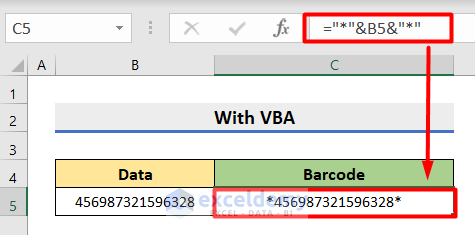
First, insert this formula for the data 456987321596328 and press Enter.
="*"&B5&"*"Then, change the Font to Code 128 and the Size to 36 for creating the barcode.
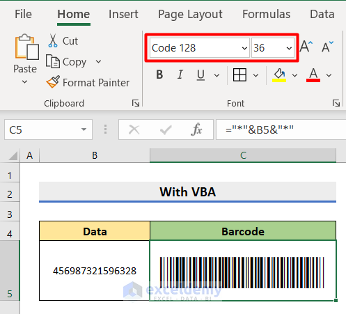
Make sure, your input data is in Text format before applying the formula.
Moreover, VBA is not error-free. So I suggest you create a new Excel-Macro Enabled Workbook and copy-paste the VBA code to create your own barcode.
I hope this will help you to solve your problem. Please let us know if you have other queries.
Thanks!
Hi Muniru Tahiru,
Thank you for sharing your problem. To solve this you can go through this article. I hope it will help you.
https://www.exceldemy.com/automatically-update-one-excel-sheet-from-another-sheet/#top_ankor
Please let us know if you have other queries.
Thanks!