How to Create Many to Many Relationship in Excel

When we work with multiple data strings in different worksheets, we often need to merge them. It is mostly required to get an overall view of the whole workbook. To do this, Microsoft Excel has introduced Power Pivot to interlink all excel tables and the process is called many to many relationship. In this article, we will guide you on how to create many to many relationship in excel through some easy steps.

What Is Many to Many Relationship in Excel?

When we interlink two or more tables based on one or more common items, then it is called the many to many relationship. It helps to fetch complicated information that has repetitive values in different scenarios.

People mostly adapt a many to many relationship for business forecasting, production control, analyzing decades of data, etc.

Types of Relationships Between Tables in Excel

In Excel, we can create three different types of relationships among tables. They are:

1. One to One: Only a single record is related between two tables.

2. One to Many: A single record of one table is connected to multiple records of another table.

3. Many to Many: Multiple records of each table are related to each other.

How to Create Many to Many Relationship in Excel: Step-by-Step Procedures

Now, we are at the main part of our article. Following we will discuss the process to create a many to many relationship between two tables with just 6 steps.

STEP 1: Create Table with Dataset

To start the process, we need to have datasets and convert them into excel tables.

First, create a dataset in the Cell range B4:D19 of a company’s Sales Report in October 2022.

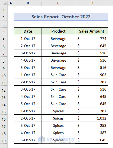
Similarly, prepare another dataset of Profit Report.

Now, select the Cell range B4:D19 in the first worksheet.
Then, go to the Home tab and click on Format as Table.

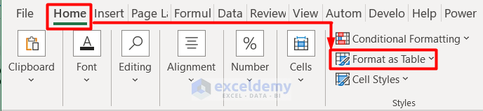
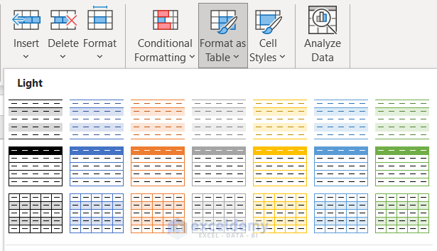
Afterward, choose any style for the table.

Finally, you will get the dataset as a table like this.

Along with it, follow the same procedure for the Profit Report worksheet as well.

STEP 2: Add Tables to Power Pivot

Now, we will insert the table into the Power Pivot. It is the ultimate analysis tool in excel for a dynamic data model. To do the task, follow the process below.

In the beginning, we will install the Power Pivot add-in to our workbook.
For this, go to the File > Options tab.
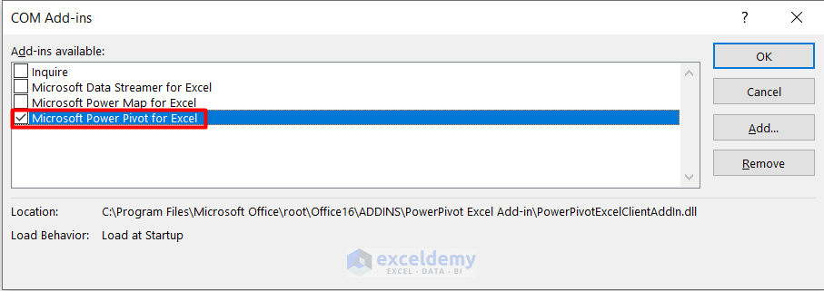
Then, COM Add-ins under the Add-ins section and press Go.

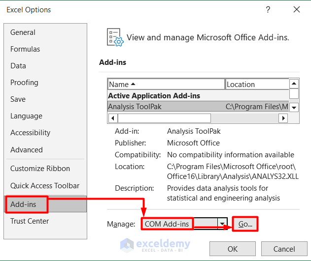
Next, select Microsoft Power Pivot for Excel and press OK.

Now, select the first worksheet.
Then, go to the Power Pivot table in the Excel Ribbon and select Add to Data Model.

Along with it, do the same for the second worksheet as well.
Finally, you will get both tables in the Power Pivot window.

STEP 3: Create Pivot Table from Power Pivot

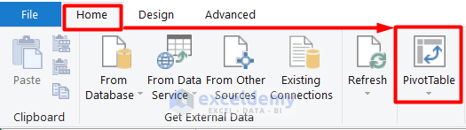
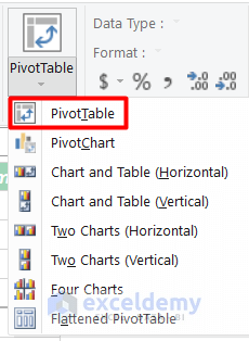
At this stage, we will create a Pivot Table to get summarized data from the Power Pivot. Let’s see how it works.

Firstly, select PivotTable from the Home tab in the Power Pivot window.

Secondly, choose PivotTable from the drop-down menu.

In the following step, choose the location of the Pivot Table.
As we want it in another worksheet, that is why we choose New Worksheet.
Afterward, press OK.

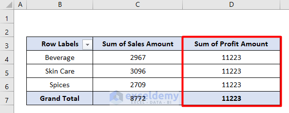
Next, put the categories in respective fields under the PivotTable Fileds panel as shown below.

Afterward, you will see that Sum of Profit Amount is showing inaccurate values.

To find the reason, go to the Diagram View in the Home tab of the Power Pivot window.

Here, connect the Date title of both tables by dragging the cursor all over them like this.

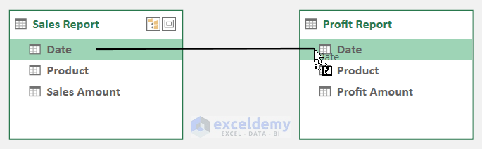
Lastly, you will get this warning message which states that the relationship cannot be created due to duplicate values.

STEP 4: Produce Date Table in Excel

This error occurs because both tables have duplicate values like Date and Product. As they are interrelated yet, we will create a separate Date table to solve this.

In the beginning, open a new worksheet with the Date values only.
Then, insert this formula in Cell C5 to get the Month value and press Enter.

=MONTH(B5)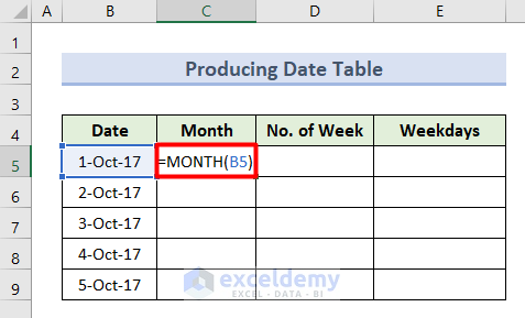

Here, the MONTH function pulls out the month number from Cell B5 in a numeric format between 1 to 12.

Then, insert this formula in Cell D5 for getting the No. of Week for the respective date and hit Enter.

=WEEKNUM(B5)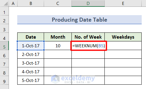

In this formula, the WEEKNUM function returns the specific week number of the given date in Cell B5.

Similarly, type this formula in Cell E5 for counting Weekdays and press Enter.

=WEEKDAY(B5,2)

The WEEKDAY function returns the specific day of the week from the reference Cell B5.

Finally, you will get details Date Table like this.

Lastly, apply the AutoFill tool to get individual parameters for all the dates.
Also, press Ctrl + T to convert it into a table.

STEP 5: Insert Many to Many Relationships Between Tables

Finally, we are at the stage, where we will create the many to many relationship between the tables. To do this, follow the process below.

In the beginning, add the Date Table to the Power Pivot following the process in Step 2.

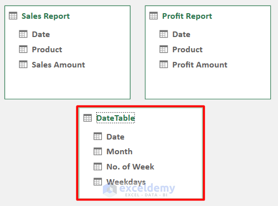
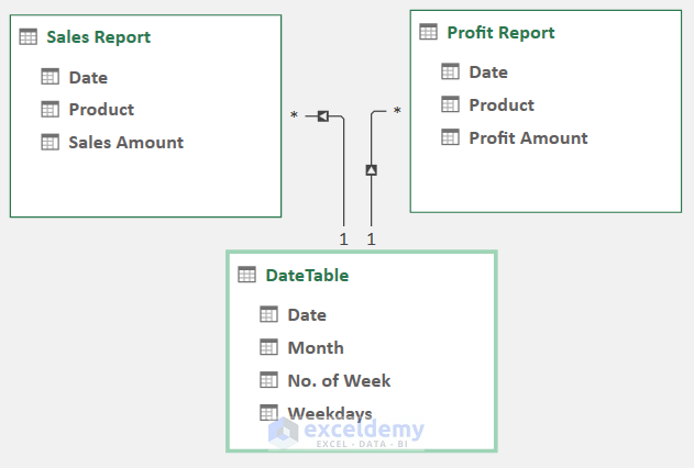
Then, connect the Date titles of the Sales Report and Profit Report tables with the Date Table by dragging the cursor like this.

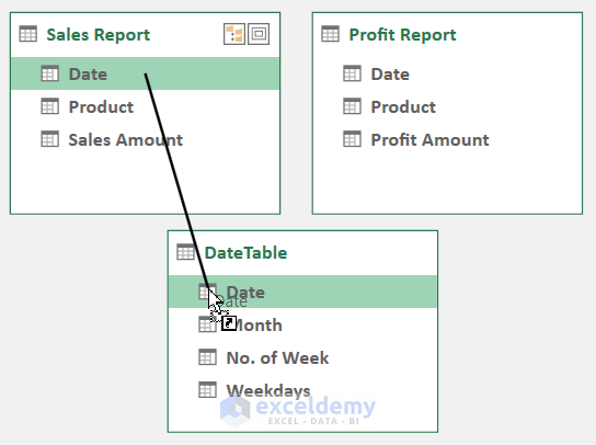
Finally, you will see the connection strings which define that the tables have many to many relationship.

STEP 6: Get Final Output in Pivot Table

To view the final output, follow the process below.

Initially, go to the Pivot Table that we created earlier.
Then, drag Weekdays to the Rows field.

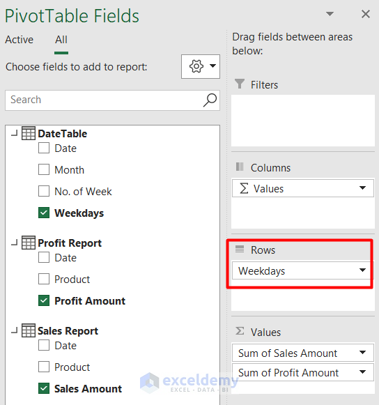
Finally, you will see that the Pivot Table is showing the accurate values which means we have successfully created many to many relationship among the tables.

Follow the same procedure for other categories as well.

Download Practice Workbook

Download this sample file and practice by yourself.

Create Many to Many Relationship.xlsx

Conclusion

Henceforth, we are concluding our article on how to create many to many relationship in excel. Here we described the process with easy steps for your better understanding. Let us know your insightful suggestion on this.

<< Go Back to Create Relationships in Excel | Data Model in Excel | Learn Excel

Get FREE Advanced Excel Exercises with Solutions!