Latest Posts From Alif Bin Hussain

Volatility is the speed and magnitude of the fluctuations of the price of a specific time period. The price of an asset or a commodity might change every day ...

Method 1 - Create a VBA Dictionary Steps: Open the Microsoft Visual Basic window by pressing Alt+F11 . Click on the Tools tab and go to, Tools → ...

We will use the following dataset to demonstrate how to make a rating scale. It has a number of products and a rating score for each of them. Method ...

Here’s an overview of the dataset for today’s article. Step 1 - Create Borrower and Lender Columns Create two columns with Borrower and Lender ...

We will demonstrate 10 useful techniques to navigate large Excel spreadsheets. We will use the following dataset. Method 1 - Use the Zoom Level ...
Method 1 - Calculate Material Cost for Residential Construction Create columns named No. and Materials to add numbers and names of materials. We need ...
Method 1 - Using the Accent Option Click the Insert tab. Click on Symbols followed by Equation. Choose Accent and select Bar. A text ...
Introduction to Skewness and Kurtosis Skewness Skewness is a measure of the level of asymmetry in the distribution of a dataset. When a dataset is not ...
Step 1 - Create a Dataset with Proper Parameters Create your dataset in Excel. We created a column of Sales Representatives names with two other columns of ...

Method 1 - Use VBA Code to Display Tooltip on Mouseover for Text Steps: Display tooltips for the Sales Rep To do it, press Alt+F11 . Open the ...

This is the sample dataset. Method 1 -Using Basic Shapes to Circle a Text in Excel Steps: Go to the Insert tab and click Shapes. Select ...
Method 1 - Create a Dataset with Proper Parameters Create your list. We created a "List of Food" column with 8 items and another column with “Quantity Sold." ...

While dealing with a graph of a curve in Excel, an individual might need to determine the instantaneous slope of any specific point on the curve. This ...

Excel can be very helpful in determining remainders. One might need these remainders in Integer or in decimal format. In this article, we will show you how to ...
Method 1 - Add a Text Box using the Insert Tab Steps: Go to the Insert tab. Click Text Box.. The cursor will show a cross. ...
See Our Reviews at


Hello FAIS,
Follow these steps to get your desired result.
=LN(C6/C4)/LN(1+C5)In the formula, C6 refers to the desired salary (75000000), C4 refers to the current salary (307584) and C5 refers to the increment percentage (10%).
=INT(C8)&" years " & INT(MOD(C8*12,12))&" months"Here, C8 refers to the required time in years.
Hello Tom,
The upward arrow between C9 and C10 in the formula indicates the exponent operation of mathematics. In the formula, C9 raised to the power of C10 is written as C9^C10. A simple example would be “Two Squared” which is written as 2^2 = 4, where 2 is raised to the power of 2, resulting in 4.
Hello Claire,
Follow these steps to make the stacked bar charts of Likert scales.
Insert >> Charts >> 100% Stacked Column
Hello Torsten,
Thank you for bringing this matter to our attention. We will look into the VBA function to see if it can be updated to minimize the deviation of the orange line from the given points.
Besides, I would like to address your concern regarding interpolation methods. There are some interpolation methods that go through all the given points such as Lagrange interpolation or polynomial interpolation etc. However, interpolation method such as cubic spline interpolation does not necessarily pass through all the given data points.
Hello SANJAY DANGI,
Thank you for reaching out. You can add attachment to the email in the first method easily. Follow these steps to do it.
Sub ExcelToOutlookSR() Dim mApp As Object Dim mMail As Object Dim SendToMail As String Dim MailSubject As String Dim MailBody As String Dim FileName As String Dim Path As String 'Declare variable for file path Path = "D:\Exceldemy\" 'Set file path For Each r In Selection SendToMail = Range("C" & r.Row) MailSubject = Range("F" & r.Row) MailBody = Range("G" & r.Row) FileName = Range("H" & r.Row) 'Get file name from H column Set mApp = CreateObject("Outlook.Application") Set mMail = mApp.CreateItem(0) With mMail .To = SendToMail .Subject = MailSubject .Body = MailBody .Display .Attachments.Add (Path & FileName) 'Add attachment End With Next r Set mMail = Nothing Set mApp = Nothing End SubHello Theo,
Follow these steps to adjust ranges to make a longer list without any error.
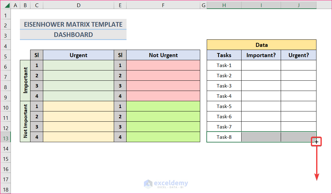
1. First, to make the task list longer, select cells H13 through J13. Then drag the fill handle down to add new task.
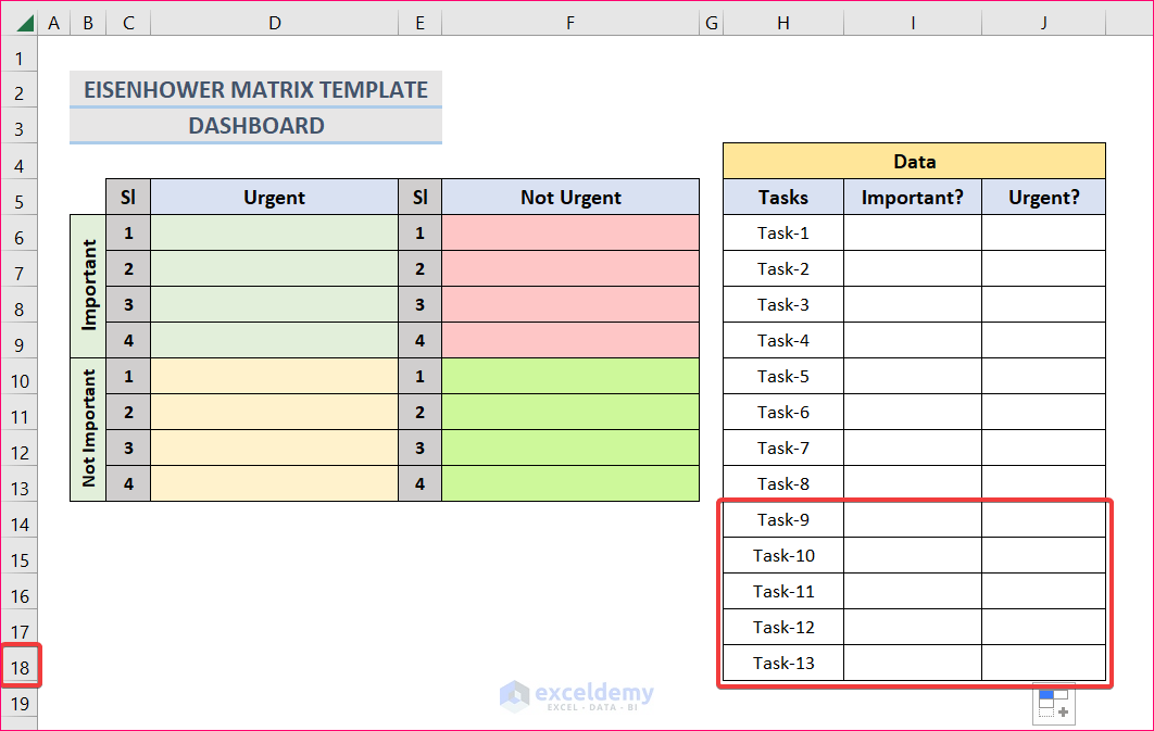
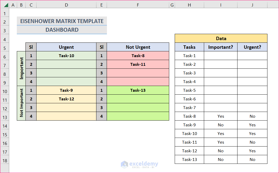
2. In this example, we added five new tasks. Therefore, the new ranges for column H, I and J are H6:H18, I6:I18 and J6:J18 respectively.
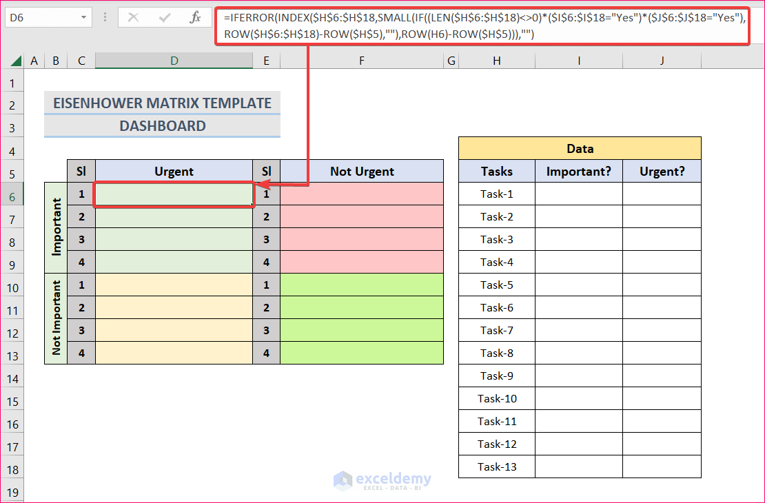
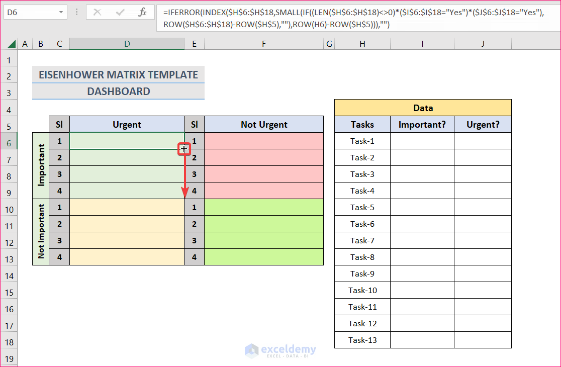
3. Then select cell D6 and change the ranges of H,I and J cells in the formula bar and press Enter. After that, Autofill formula up to cell D9.
4. Similarly, change the formula ranges for other cells as well.
5. Finally, you can see in the following figure that the formula is working properly.
I hope this solves your problem. Please let us know if you face any other issues.