How to Navigate Large Excel Spreadsheets (10 Useful Techniques)

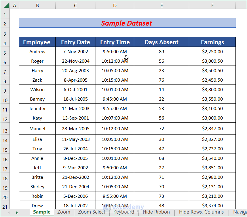
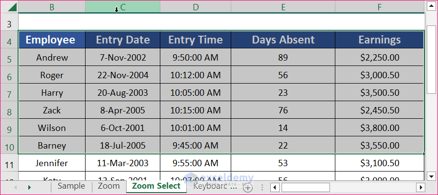
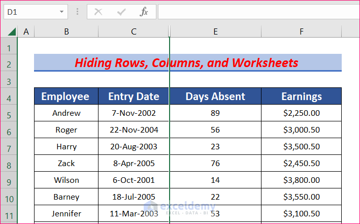
We will demonstrate 10 useful techniques to navigate large Excel spreadsheets. We will use the following dataset.

Method 1 – Use the Zoom Level Feature for Navigating Large Excel Spreadsheets

Steps:

• Go to the bottom-right corner of the program.
• Click on the “-” sign to zoom out.

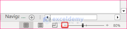
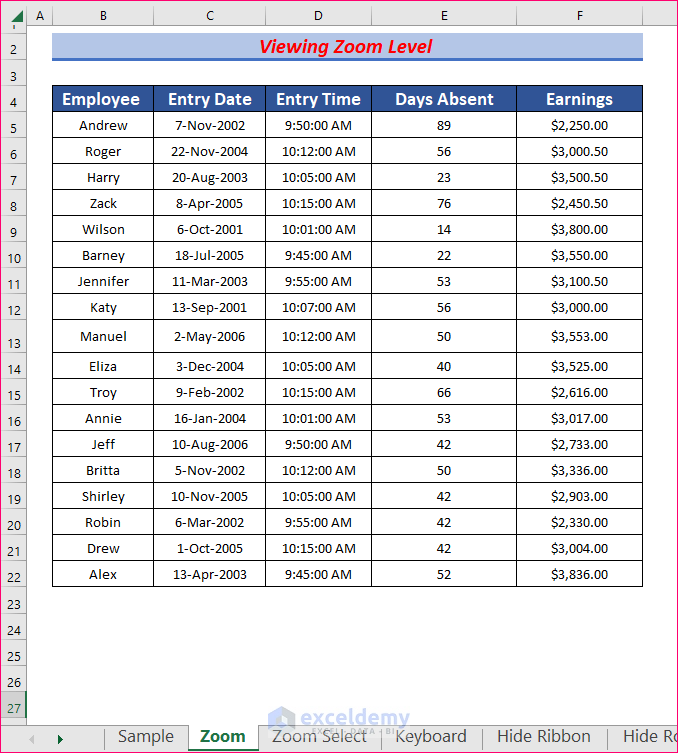
• Keep clicking the sign until you can see more values.

Method 2 – Apply the Zoom to Selection Feature

Steps:

• Select the cells you want to zoom in on.
• Click on the View tab and go to Zoom, then select Zoom to Selection.

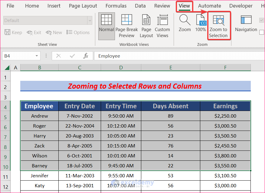
• You will find the selected cells zoomed in on the window.

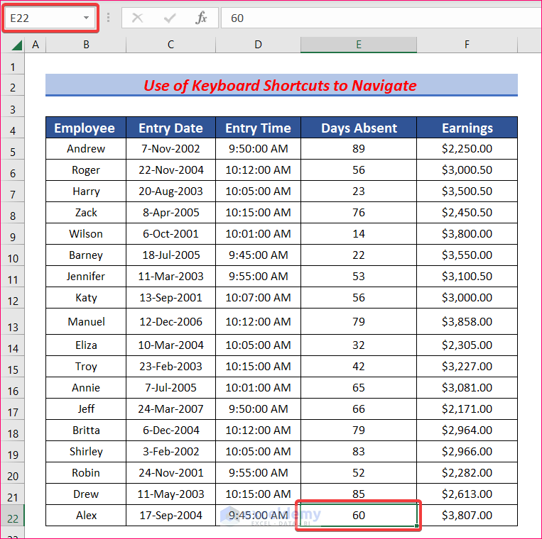
Method 3 – Use Keyboard Shortcuts for Navigating Large Excel Spreadsheets

Steps:

• We want to go to the last non-zero cell of any row.
• Select any of the cells of that row.

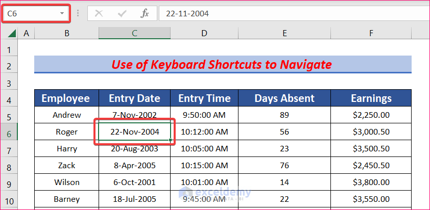
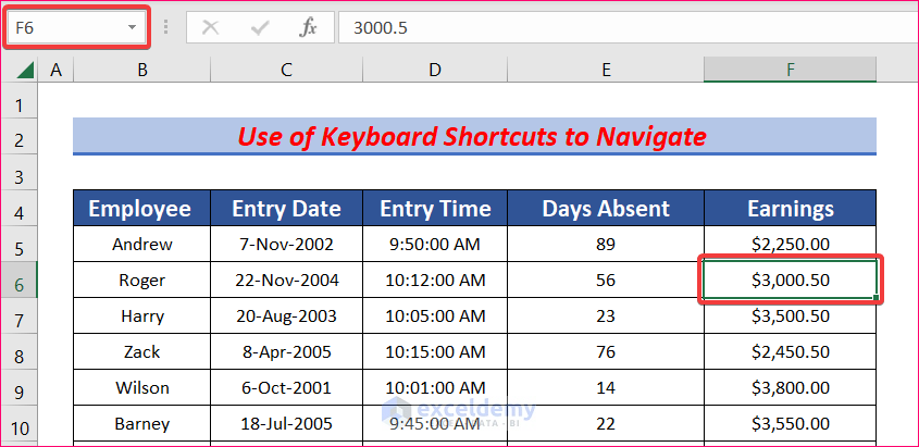
• Press Ctrl + Right Arrow to get to the rightmost non-zero cell in that row.

• To go to the last cell of a column, select any cell of that column.

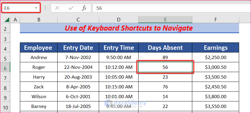
• Press Ctrl + Down Arrow to move to the last non-zero cell of that column.

Method 4 – Hide the Ribbon for Navigating Large Excel Spreadsheets

Steps:

• Right-click the ribbon anywhere.
• Select Collapse the Ribbon to hide the ribbon.

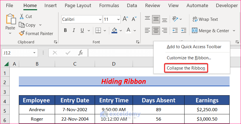
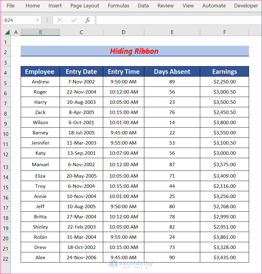
• Here’s the result.

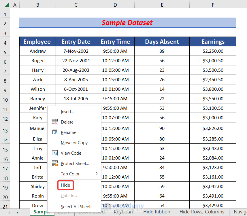
Method 5 – Use the Hide Option to Hide Rows, Columns, and Worksheets

Steps:

• Select the column or row you want to hide.
• Right-click on the column or row and select the Hide option.

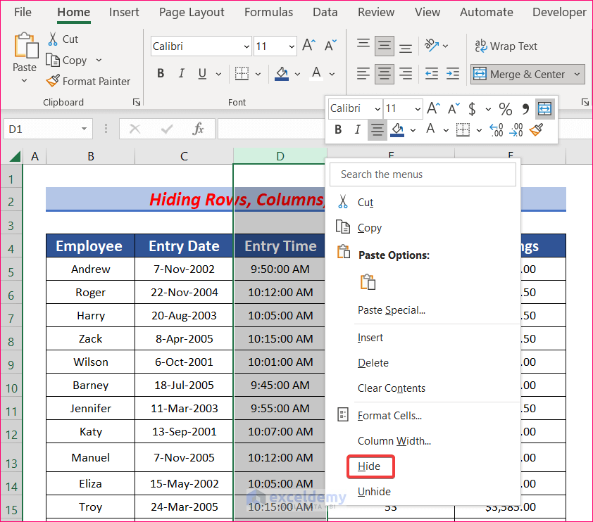
• Once you click on Hide, the column or row will be hidden.

• To hide a worksheet, right-click on the worksheet and select Hide.

The worksheet is hidden.

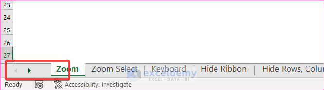
Method 6 – Navigate Worksheets

Steps:

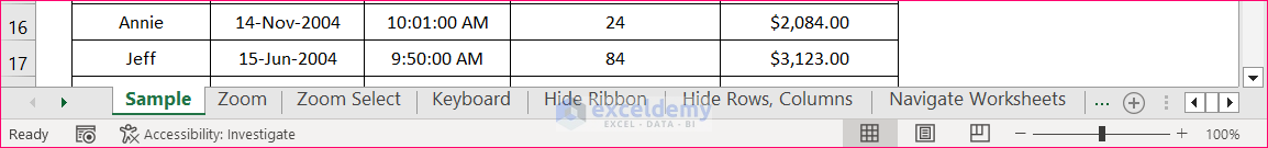
• Move your cursor to the bottom-right corner of the window.
• Click and drag the “three dots” to the right until all the worksheets are visible.

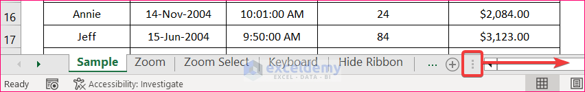
• You can see all the tabs and can navigate them with one click.

Read More: How to Navigate Between Sheets in Excel

Method 7 – View Worksheets Side-by-Side

Steps:

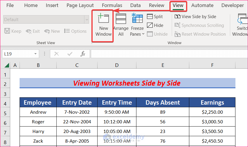
• Click on the View tab and go to Window and select New Window

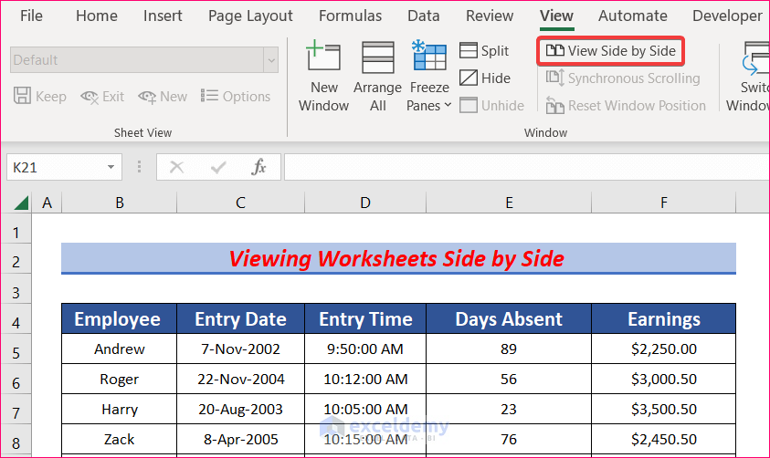
• A new window will appear. Select View Side by Side.

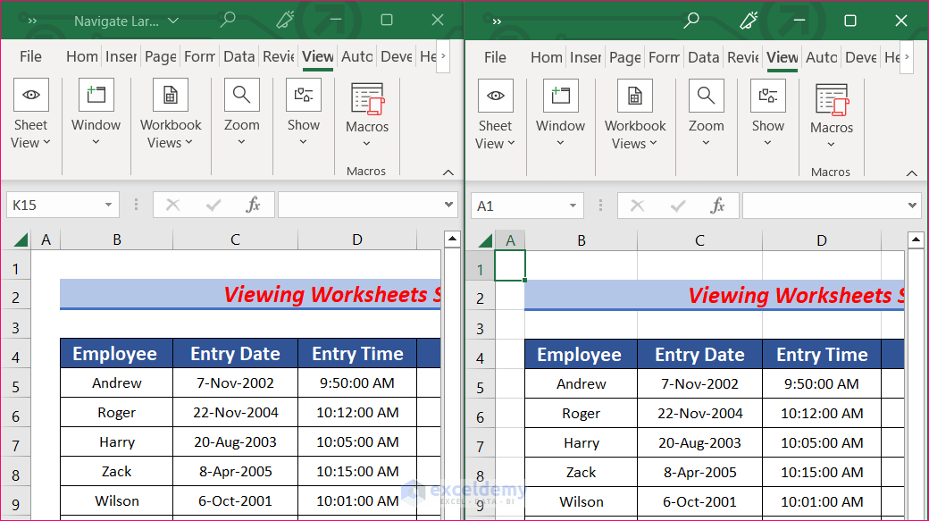
• You will have two Excel windows side by side.

Method 8 – Freeze Rows and Columns

Steps:

• Select the row below the one you want to be frozen.
• Open the View tab and go to Freeze Panes.
  

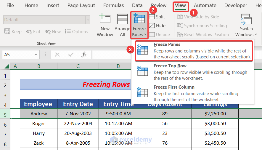
• Select Freeze Panes.
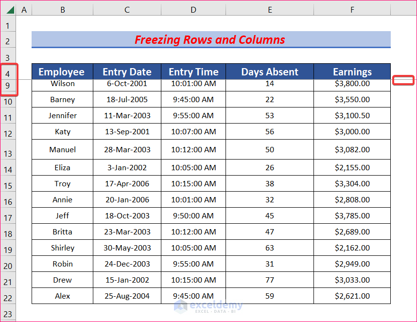
• You will see a straight line over the row you previously selected. Above this line, the rows are frozen.
• If you want to freeze both row and columns, select the cell in the row and column after the ones you want to freeze.

Read More: How to Use Navigation Pane in Excel

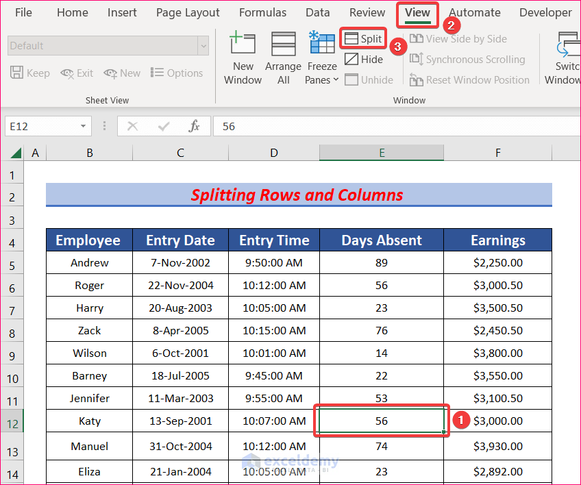
Method 9 – Split Rows and Columns

Steps:

• Select a cell that is situated just right and bottom to the splitting point. The top left corner of the cell is the same point as your chosen point to split.
• From the View tab go to Split.

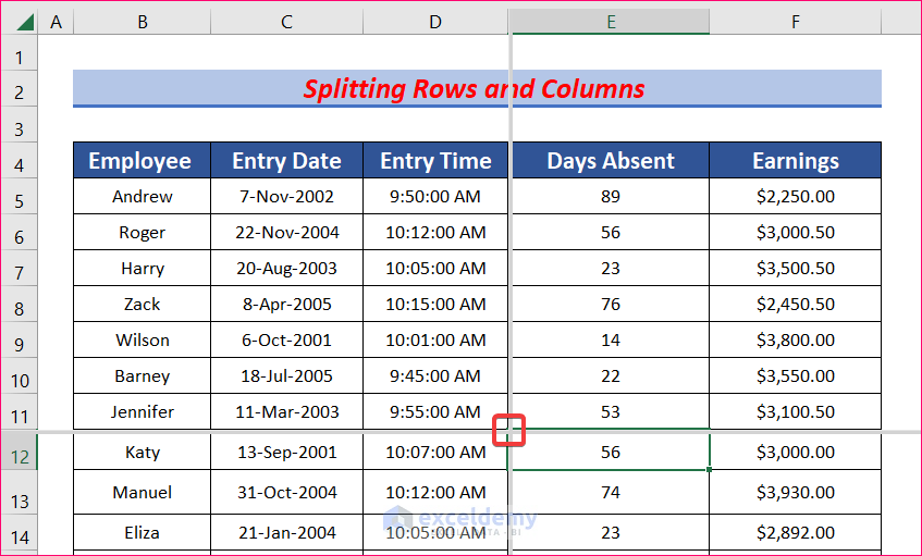
• You will get your sheet split into four segments.

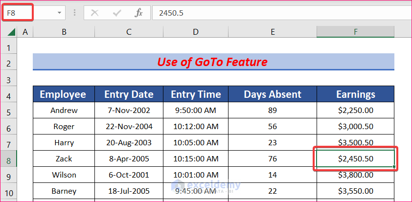
Method 10 – Use the Go To Feature for Navigating Large Excel Spreadsheets

Steps:

• Press F5 on your keyboard.
• A pop-up box will open. Type your desired cell reference and hit Enter.

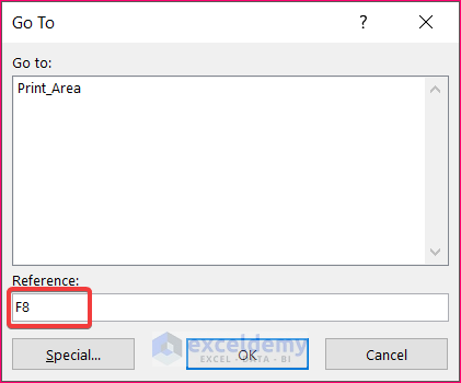
• You will go to the desired cell.

Download the Practice Workbook

Related Articles

• How to Create Navigation Buttons in Excel
• [Fixed] Excel Navigation Arrow Keys Not Working
• How to Perform Cell Navigation in Excel
• How to Perform Tab Navigation in Excel
• How to Use Navigation Keys in Excel

<< Go Back to Navigation in Excel | Learn Excel