How to Use Navigation in Excel?

In this article, you will learn how to
-Navigate within Excel cells and worksheets
-Move across selected ranges for navigation
-Use the scroll lock and scroll bars for navigation
-Use the Navigation Pane for charts and tables in Excel

We have used Microsoft 365 to prepare this article. But these methods apply to Excel 2021, 2019, 2016, 2013, 2010, and prior versions.

We will use Excel navigation methods to work faster and improve efficiency while working with spreadsheets.

Download Practice Workbook

How to Use Navigation Shortcuts in Excel? (9 Easy Ways)

Here, we will show you nine different types of navigation shortcuts in Excel. We will use these navigation shortcuts to navigate across Excel cells, worksheets, rows, columns, and many more.

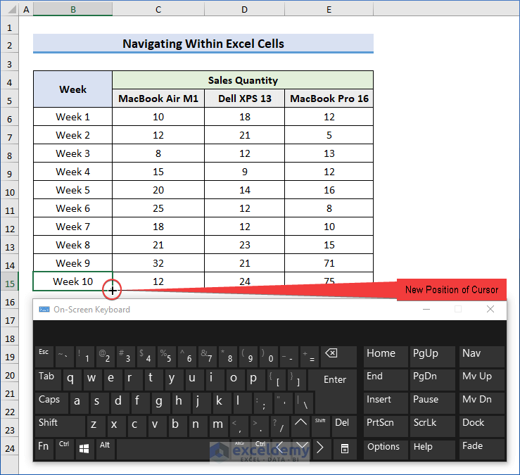
1. Navigating Within Excel Cells in Excel of a Data Region

You will learn how to move the cursor position within Excel cells to perform cell navigation. Follow the steps below.

• Firstly, select the B6 cell, which is the first row of the table ⟹ press the Ctrl + Down Arrow keys.

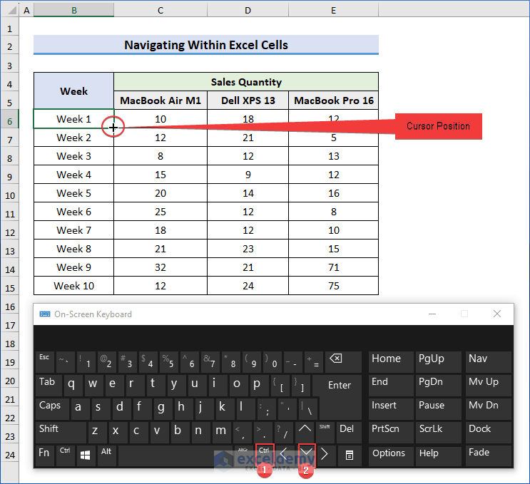
• Now, you can see the cursor is in the last row of the data region.

2. Navigating to the First Cell of the Worksheet

In this part, we will show how to navigate to the first cell of the Excel worksheet. In the image below, you can see a sample dataset where the initial cell position is in the B6 cell.

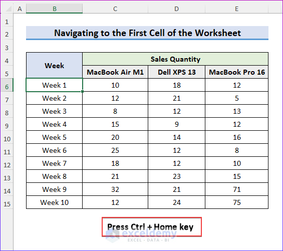
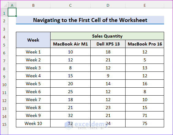
• Select the B6 cell ⟹ and press Ctrl + Home key.
• Now, it will move the cursor to the first cell (A1). 

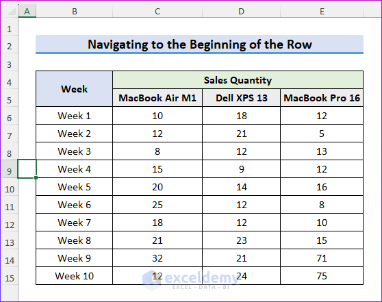
3. Navigating to the Beginning of the Row of the Worksheet

To go to the beginning of the row in the worksheet, follow the below steps. 

• Select any cell on the worksheet. We have selected the E9 cell.

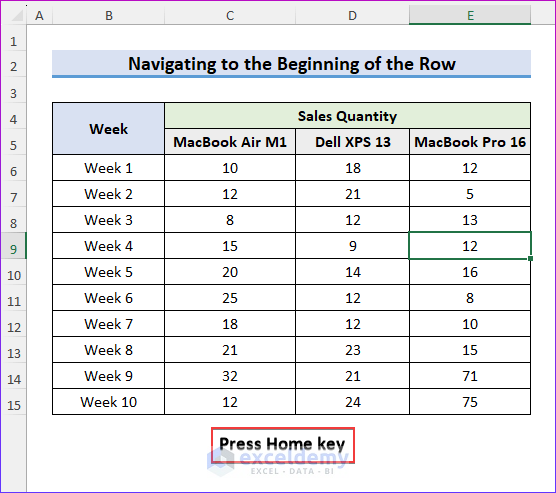
• Press the Home key.
• Finally, it will move the cursor to the beginning of the row of the worksheet in cell A9.

4. Navigating to a Specific Cell of the Worksheet

In this part, we will show how you can navigate to a specific cell from the Go To dialog box.

• Press F5 or Ctrl + G to open the Go To dialog box.
• Now, write any cell address in the Go To dialog box. We have written C8 as a cell reference here.

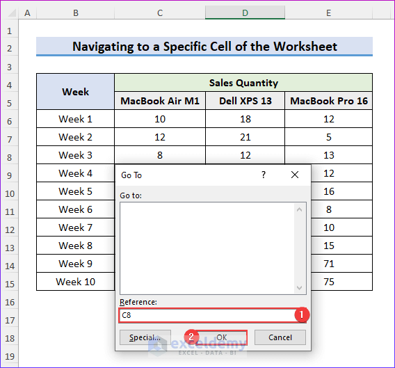
• Finally, you can see that it will select the C8 cell that you wrote in the Go To dialog box.

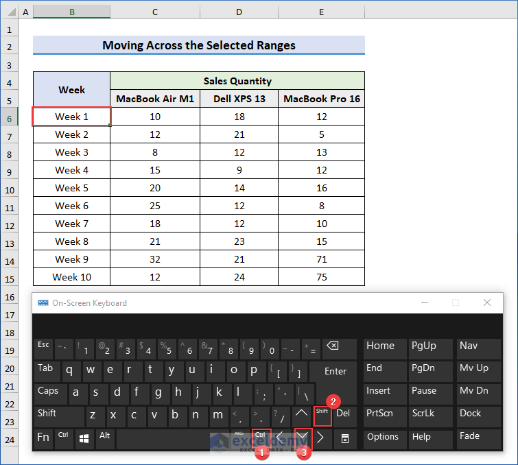
5. Moving Across Selected Ranges for Navigation

In this section, we will show how to select any cells in a specified range.

• Go to the B6 cell ⟹ and press Ctrl + Shift + Down Arrow keys.

Click on the image for a detailed view

• Here, you can see that all the cells in range B6:B15 have been selected. Now, press the Tab key on the keyboard.

Click on the image for a detailed view

• When you press the Tab key, it will move the cursor from the top by one cell within the selected range.

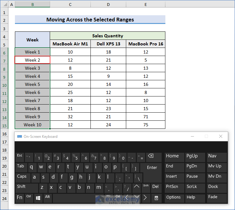
Click on the image for a detailed view

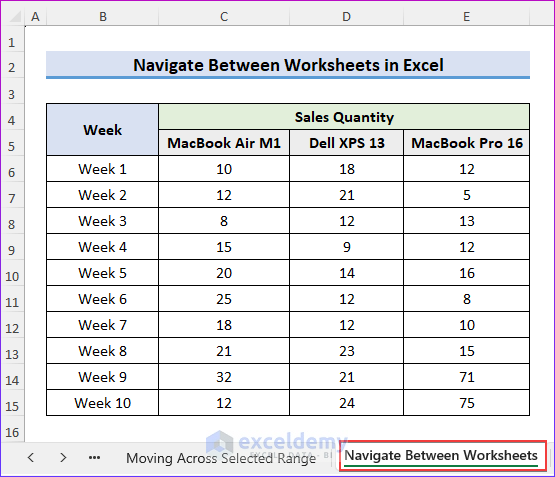
6. Navigating Between Worksheets in Excel

It is necessary to navigate worksheets in Excel when you work with multiple sheets. To learn how to do it, follow the steps below.

• This is our main worksheet named “Navigate Between Worksheets”.
• If you want to switch between two sheets, click on the Ctrl ⟹ PgUp keys, and it will move to the previous worksheet. 

• Now, you will see the previous worksheet named “Moving across Selected Range”.

• And, when you click on the Ctrl ⟹ PgDn keys, it will move back to the main worksheet.

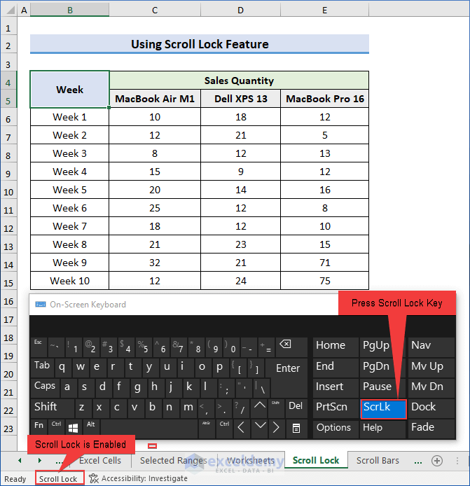
7. Using the Scroll Lock Feature to Navigate Between Pages

You can scroll between pages to maintain large sets of data by enabling the Scroll Lock feature

• Press the ScrLK (Scroll Lock) button to enable scroll lock which helps you to scroll large pages. You will see a scroll lock enabled in the status bar.

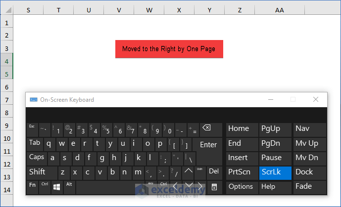
• Now, press the Ctrl ⟹ Right Arrow key as shown in the image below.

• Finally, the screen is shifted to the right by one page.
• Similarly, you can move back to the left by one page by pressing the Ctrl ⟹ Left Arrow key.

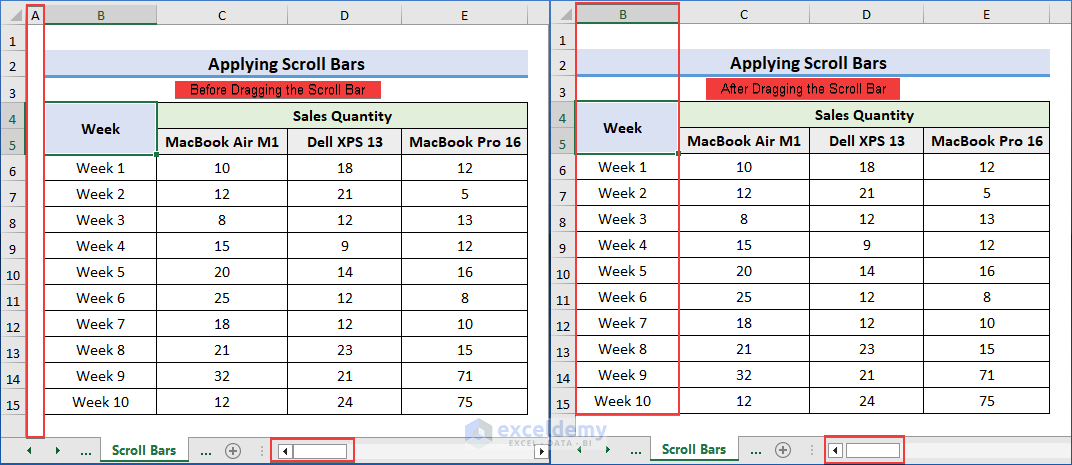
8. Applying Scroll Bar for Left-Right Navigation in Excel

Here, we will look at moving rows and columns using the Scroll Bars in Excel.

• Drag the Scroll Bar from left to right.
• After dragging, you can see the dataset moved to the left by one column.

Click on the image for a detailed view

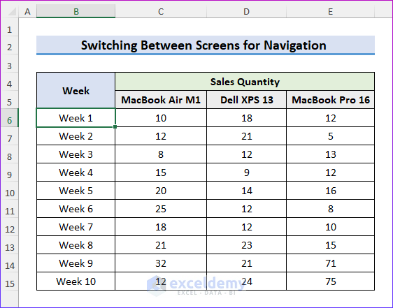
9. Switching Between Screens for Navigation in Excel

In this part, we will show you how to switch from one screen to another on your device. It may vary with your monitor size.

• Select the B6 cell ⟹ and press the Page Down key.

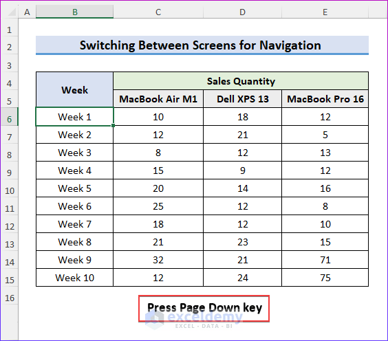
• Now, it will move to the next screen of the B33 cell. So, it switches to one screen from row 6 to row 33.

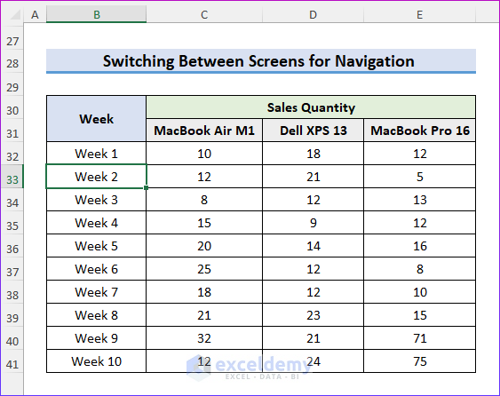
• Again, by pressing the Page Up key, it will move back to the B6 cell.

How to Use Navigation Pane For Charts, and Tables in Excel?

In this part, we will use the navigation pane to navigate charts and tables in Excel.

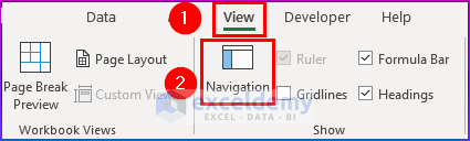
• Firstly, go to the View tab, then click on the Navigation Pane.

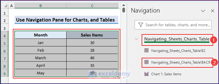
• Now, select any sheet that you want to navigate and their charts, datasets, tables, etc.
• Then, you will see different elements of that worksheet displayed in the navigation pane.
• Here, we have selected Navigating_Sheets_Charts_Table ⟹ Navigating_Sheets_Charts_Table!B4:C9 and it takes us to the dataset of the worksheet.

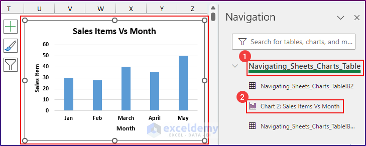
• Now, we have selected range B4:C9 of the sheet named Navigating_Sheets_Charts_Table ⟹ Chart 2: Sales Item Vs Month and it will select the graph.

Things to Remember

• Enabling Scroll Lock allows smooth scrolling through the worksheet without changing the active cell. This is particularly useful when dealing with large datasets.
• Always double-check that you’ve selected the correct cells before performing any action. Selecting the wrong cells can lead to unintended changes in your data.
• Be cautious when navigating through sheets with hidden rows or columns. Hidden data can affect calculations and analysis. Unhide them when necessary.
• The sheet tabs at the bottom of the Excel window make it easier to switch between worksheets in a workbook.

Frequently Asked Questions

1. Can I create custom-named ranges for easy navigation in Excel?

Yes, you can define named ranges to make navigation easier. Go to the Formulas tab, and click on Name Manager to create a new named range. Then, you can navigate to that named range by using Ctrl + G and selecting the range from the list.

2. How do I switch between different open workbooks using the keyboard?

You can use the “Ctrl + F6” shortcut to cycle through different open workbooks. Press “Ctrl” and then repeatedly press “F6” to switch between them.

3. How can I quickly move to the start or end of a row or column?

Press the Ctrl + Arrow key to move to the last filled cell in that direction. For example, the Ctrl + Down Arrow key will take you to the bottom of the current column.

4. How can I make an Excel navigation link?

• Create a Link to a website
• Choose the cell on a worksheet where you want to link something.
• Insert tab ⟹ Hyperlink button.
• Enter the text you want to use to represent the link under Display Text.
• Enter the complete Uniform Resource Locator (URL) of the website you want to connect to under the URL.
• Choose OK.

Conclusion

In this article, we have demonstrated various applications of the navigation shortcuts in Excel to navigate across Excel cells, worksheets, rows, columns, and many more.  You can navigate any size spreadsheet more quickly and precisely by using the shortcut and navigation keys in Excel. We have also discussed their examples and usages with proper explanations. Further, you will learn the basics of how to use the navigation pane for navigating charts and tables in Excel from this article.

We hope you find this helpful article. If there are any further queries or recommendations, feel free to comment.

Navigation in Excel: Knowledge Hub

• Create Navigation Buttons
• Navigate Large Excel Spreadsheets
• Use Navigation Keys
• Perform Tab Navigation
• [Fixed] Excel Navigation Arrow Keys Not Working
• Scrolling in Excel
• How to Turn On/Off Scroll Lock in Excel

<< Go Back to Learn Excel