The navigation pane in Excel is a helpful tool that provides a quick and organized way to navigate through the various elements within your workbook. The navigation pane allows you to easily manage and move between sheets, tables, charts, and other objects within your workbook. Instead of scrolling through the entire workbook, you can use the navigation pane to jump straight to where you want to be.
It’s super useful when you’re working with big and complex data because it saves time and makes things much easier. Just open the navigation pane, click on what you’re looking for, and Excel will take you there in a snap!
In this article, we will show three handy applications on how to use the navigation pane in Excel.
In the following GIF, I have used the Navigation Pane to navigate through different elements, including the range of cells, charts, and headings.
How to Open the Navigation Pane in Excel
In Microsoft Excel, the Navigation Pane is a feature that helps users navigate and manage the elements within a workbook. It was introduced in Excel 2013 and is particularly useful when working with large and complex workbooks.
To open the Navigation Pane, go to the View tab of the Excel ribbon and select Navigation.
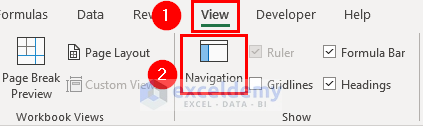
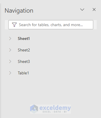
As a result, you will see the navigation pane on the right side of the worksheet.
3 Simple Applications of Using Navigation Pane in Excel
Finding your way around the Excel workbook has become quite accessible since the introduction of the navigation pane. With the help of a navigation pane, we can find different elements of the workbook easily. Also, it’s possible to perform different actions on those elements.
The navigation pane has different applications with worksheets and their elements. Here, we will discuss three handy applications of the navigation pane. For demonstration purposes, we have used a few worksheets that have elements like tables, pictures, and charts.
To learn how to use the navigation pane for various purposes, follow the three applications below:
Navigating Excel Sheets, Charts, Tables, or Pictures
The primary function of the navigation pane is the easy accessibility of the worksheets and their elements.
To find your way around the workbook using the navigation pane, follow the steps below:
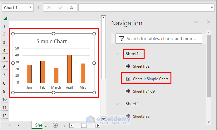
- You can select any worksheet name from the navigation pane.
- As a result, you will see different elements of that worksheet displayed in the navigation pane.
- For example, we have selected Sheet1 > Chart 1 and it takes us to the chart of the worksheet.
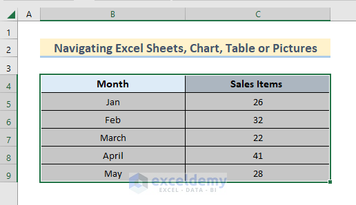
- Also, we will select the range B4:C9 of Sheet1.
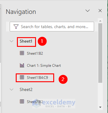
- You can see that it selects that range of cells in Sheet1.
- Now, we will select the Header of Sheet2.
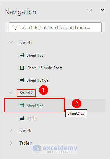
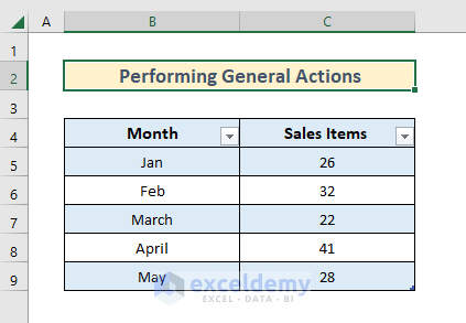
- It takes us to the Header of Sheet2.
Perform General Actions Using the Navigation Pane
Some general actions, like renaming, deleting, and hiding or showing sheets, can be done with the help of the navigation pane.
To perform those general actions using the navigation pane, you can follow the cases below:
Case 1: Renaming the Worksheet
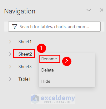
To rename the Excel worksheet, follow the instructions given below:
- Right-click on a sheet name.
- Then, select Rename from the options.
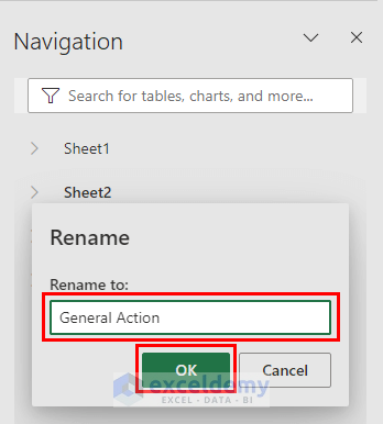
- In the Rename to box, write the new name and press OK.
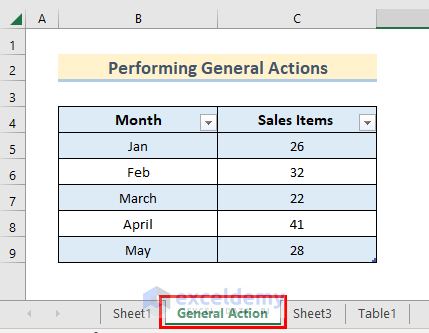
You will see the sheet name has been changed in the following image.
Case 2: Deleting the Worksheet
On the other hand, you can also hide a sheet similarly. To perform this action, follow the steps below:
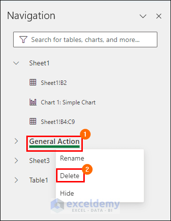
- Right-click on a sheet name. In this case, we want to delete the General Action sheet from the workbook.
- Click on Delete.
Now, you will see that the General Action sheet has been deleted from the sheet tabs.
Case 3: Hiding or Showing Worksheet
To learn how to hide or show any particular worksheet in the workbook, follow the given steps:
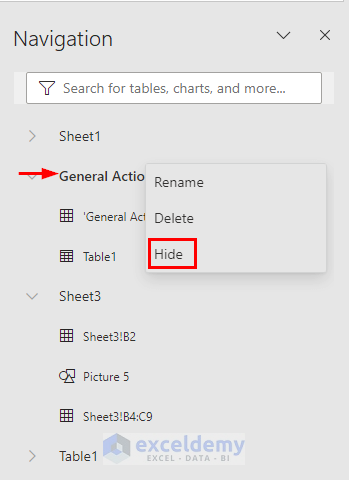
- Again, right-click on a sheet name.
- Select Hide.
 Now, the sheet name with its content is greyed out.
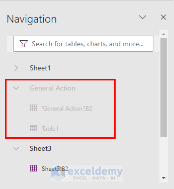 Finally, you won’t find the sheet in the sheet tab.
- Now, right-click on the hidden sheet (greyed-out sheet).
- Click on Show.
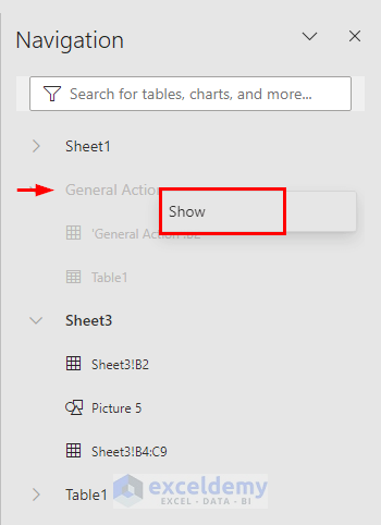 As a result, the hidden sheet will be displayed again.
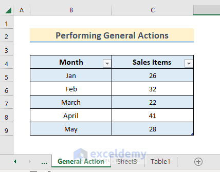
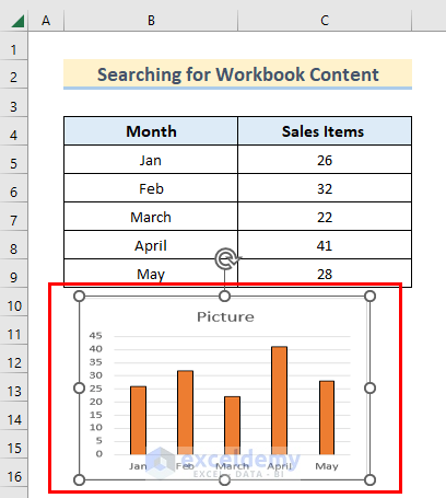
Searching for Workbook Content
Another application of the navigation pane is to search different elements of a workbook.
To search for different elements like charts, tables, or pictures from different worksheets of a workbook, follow the detailed instructions below:
- Insert the name of the element in the search box of the navigation pane. In this case, we wrote “picture.”
- The picture from any worksheet will be displayed.
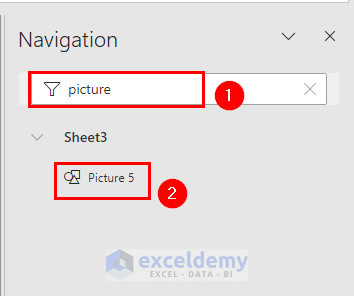
- Select that picture from the list, and it will take us to that picture in the worksheet.
- Similarly, if you want to find tables, then insert the table in the search box.
As a result, tables from the workbook will appear in the pane. - Now, select the desired table from the list in the navigation pane.
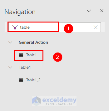
- It will take us to the table in the workbook.
Download Practice Workbook
You can download the practice workbook from here.
Conclusion
This tutorial showed various applications of the Navigation Pane. From this article, you can learn how the Navigation Pane in Excel allows users to easily navigate through different elements of their workbook, such as sheets, tables, and charts. It saves time and makes working with big and complex data much easier. If you have any questions or suggestions, let us know in the comment section.
Frequently Asked Questions
Are there keyboard shortcuts for accessing the navigation pane?
Yes, you can open the navigation pane by pressing Ctrl + F, providing a quick and convenient way to utilize this feature.
Can I customize the navigation pane to display specific elements?
While you can’t customize the Navigation Pane directly, it automatically displays a comprehensive list of sheets, tables, and charts, making it easy to find and navigate to the desired element
Does the navigation pane work in all versions of Excel?
Yes, the Navigation Pane is a standard feature in most recent versions of Excel, including Excel 2013, 2016, 2019, and Microsoft 365.
Does the navigation pane work with hidden sheets or objects?
Yes, the Navigation Pane displays all sheets and objects, including hidden ones. This allows you to access and navigate hidden elements easily.
Related Articles
- How to Create Navigation Buttons in Excel
- How to Use Navigation Keys in Excel
- How to Perform Cell Navigation in Excel
- How to Perform Tab Navigation in Excel
- [Fixed] Excel Navigation Arrow Keys Not Working
- How to Navigate Between Sheets in Excel
- How to Navigate Large Excel Spreadsheets
<< Go Back to Navigation in Excel | Learn Excel
Get FREE Advanced Excel Exercises with Solutions!
