When dealing with large amounts of data in Excel, it’s common to use INDEX-MATCH functions to look up parameters based on multiple criteria for summation or other related tasks. In this article, you’ll learn how to incorporate SUM, SUMPRODUCT, SUMIF, or SUMIFS functions along with the INDEX-MATCH formula to calculate sums under various conditions in Excel.

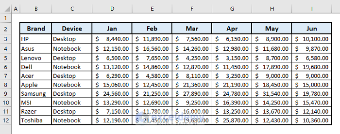
The screenshot above provides an overview of the article, showcasing a dataset and an example of how you can evaluate sums in Excel across different conditions using columns and rows. Let’s dive into the details of the functions: SUM, INDEX, and MATCH.
1. SUM
- Objective: Sums all the numbers in a range of cells.
- Formula Syntax: =SUM(number1, [number2], …)
Example:
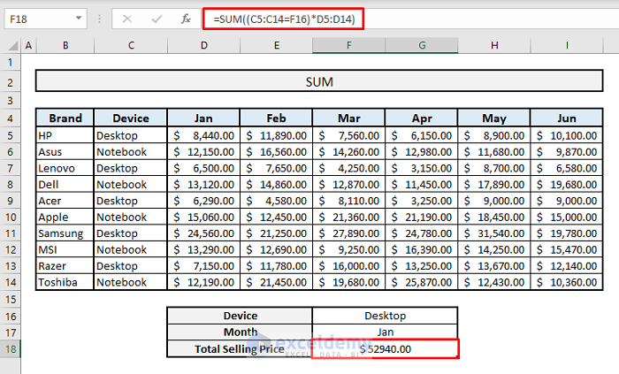
Suppose we have a dataset with a list of computer devices from different brands, along with their selling prices for six months in a computer shop. We want to find the total selling price of desktops for January only.
➤ In Cell F18, type the following formula:
=SUM((C5:C14=F16)*D5:D14)➤ Press Enter, and you’ll see the total selling price of all desktops for January.
Explanation:
- The SUM function uses only one array. (C5:C14=F16) instructs the function to match the criteria from cell F16 in the range of cells C5:C14. By adding another range of cells (D5:D14) with an asterisk (*) before it, we sum up all the values from that range under the given criteria.
2. INDEX
- Objective: Returns the value of a reference cell at the intersection of a specific row and column within a given range.
- Formula Syntax:
=INDEX(array, row_num, [column_num])
Or: =INDEX(reference, row_num, [column_num], [area_num])
- Example:
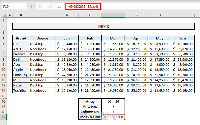
Let’s say we want to find the value at the intersection of the 3rd row and 4th column from the array of selling prices in the table.
- In cell F19, type:
=INDEX(D5:I14, 3, 4) - Press Enter to get the result.
Explanation:
- The 4th column in the array represents the selling prices of all devices for April, and the 3rd row corresponds to the Lenovo Desktop category. So, at their intersection in the array, we’ll find the selling price of Lenovo Desktop in April.
3. MATCH
- Objective: Returns the relative position of an item in an array that matches a specified value in a specified order.
- Formula Syntax: =MATCH(lookup_value, lookup_array, [match_type])
Example:
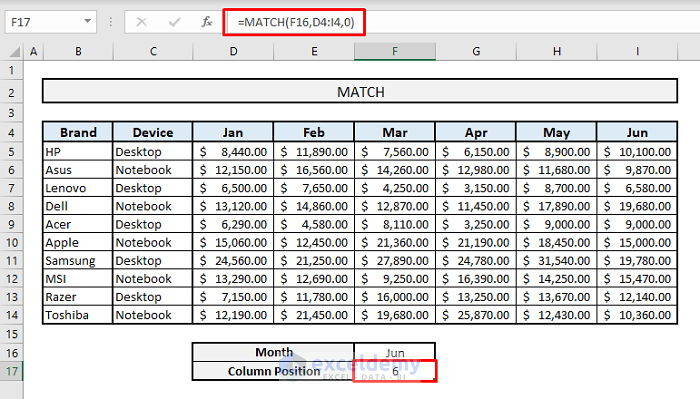
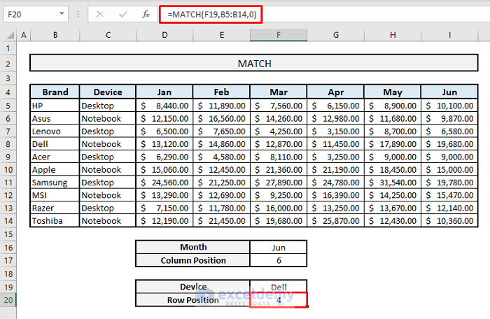
First, let’s determine the position of the month “June” from the month headers.
- In cell F17, use the following formula:
=MATCH(F16, D4:I4, 0) - Press Enter to find that the column position of June is 6 in the month headers.
Change the month name in cell F17, and you’ll see the related column position for another selected month.
Additionally, if you want to know the row position of the brand “Dell” from the brand names in column B, use the formula in cell F20:
=MATCH(F19, B5:B14, 0)
Here, B5:B14 is the range of cells where the brand name will be searched. If you change the brand name in cell F19, you’ll get the related row position for that brand from the selected range of cells.
Using INDEX and MATCH Functions Together in Excel
In this section, we’ll explore how to combine the INDEX and MATCH functions in Excel, along with examples. This combined function is effective for locating specific data within a large array. The MATCH function identifies the row and column positions of input values, while the INDEX function returns the output from the intersection of those positions.
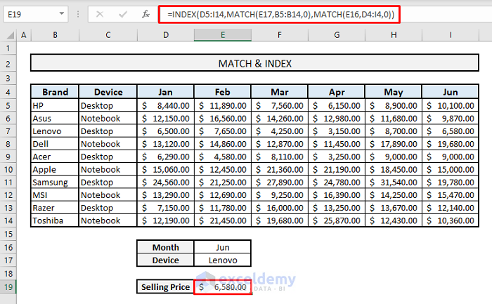
Let’s consider our dataset, and our goal is to find the total selling price of the Lenovo brand in June.
Steps:
- In cell E19, type the following formula:
=INDEX(D5:I14, MATCH(E17, B5:B14, 0), MATCH(E16, D4:I4, 0)) - Press Enter to instantly get the result. If you change the month and device name in E16 and E17, respectively, the related result in E19 will update accordingly.
Nesting INDEX and MATCH Functions inside the SUM Function
Now let’s delve into the core part of the article, where we combine SUM (or SUMPRODUCT), INDEX, and MATCH functions. By using this compound function, we can obtain output data based on ten different criteria. While we’ll use the SUM function for all criteria, you can replace it with SUMPRODUCT if needed.
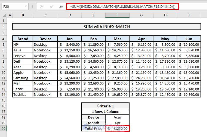
Criteria 1: Finding Output Based on 1 Row and 1 Column
For our first criterion, let’s determine the total selling price of the Acer brand in April.
- In cell F20, use the following formula:
=SUM(INDEX(D5:I14, MATCH(F18, B5:B14, 0), MATCH(F19, D4:I4, 0))) - Press Enter, and the return value will be $3,250.00.
Criteria 2: Extracting Data Based on 1 Row and 2 Columns
Next, we want to find the total selling price of HP devices in both February and June.
- In cell F21, type:
=SUM(INDEX(D5:I14, MATCH(F18, B5:B14, 0), MATCH({“Feb”, “Jun”}, D4:I4, 0))) - After pressing Enter, you’ll get the resultant value of $21,990.00.
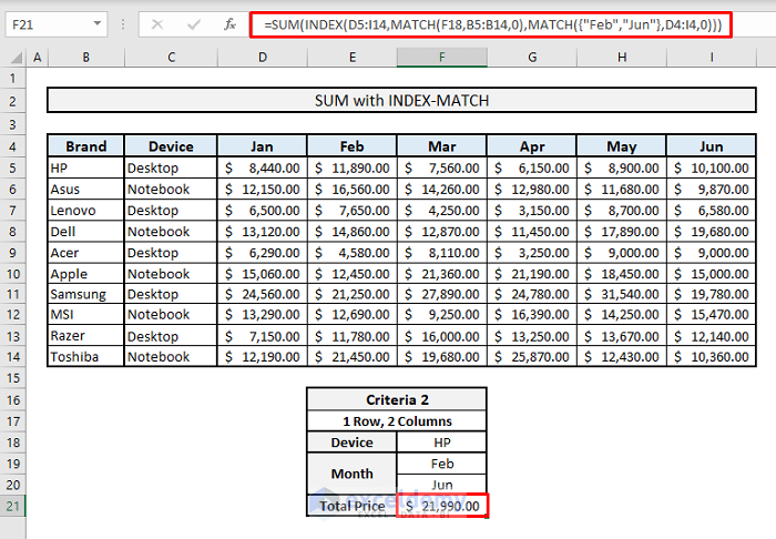
In the second MATCH function, we define the months within curly brackets, which returns the column positions for both months. The INDEX function then searches for the selling prices based on the intersections of rows and columns, and the SUM function adds them up.
Criteria 3: Determining Values Based on 1 Row and All Columns
Now let’s consider all columns with a fixed row. We’ll find the total selling price of Lenovo devices across all months.
- In cell F20, type:
=SUM(INDEX(D5:I14, MATCH(F18, B5:B14, 0), 0)) - Press Enter, and you’ll find the total selling price as $36,830.00.
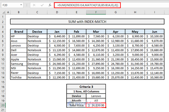
In this function, we use 0 as the argument for column position inside the MATCH function to consider all columns.
Criteria 4: Calculating Sum Based on 2 Rows and 1 Column
Finally, under the 2 rows and 1 column criteria, let’s find the total selling price of HP and Lenovo devices in June.
- In cell F21, use the following formula:
=SUM(INDEX(D5:I14, MATCH({“HP”, “Lenovo”}, B5:B14, 0), MATCH(F20, D4:I4, 0))) - After pressing Enter, the return value will be $16,680.
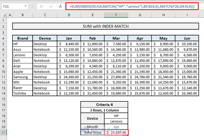
Inside the first MATCH function, we input “HP” and “Lenovo” within an array enclosed by curly braces.
Criteria 5: Evaluating Sum Based on 2 Rows and 2 Columns with SUM, INDEX, and MATCH Functions Together
In this scenario, we’ll consider 2 rows and 2 columns to extract the total selling prices of HP and Lenovo devices for two specific months: April and June.
Steps:
- In cell F22, type the following formula:
=SUM(INDEX(D5:I14,MATCH({"HP","Lenovo"},B5:B14,0),MATCH(F20,D4:I4,0)))+SUM(INDEX(D5:I14,MATCH({"HP","Lenovo"},B5:B14,0),MATCH(F21,D4:I4,0)))
- Press Enter, and you’ll see the output as $25,980.00.
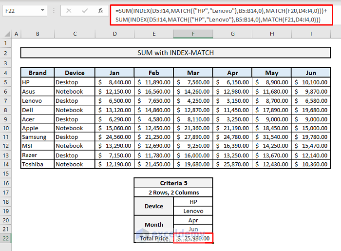
What we’re doing here is incorporating two SUM functions by adding a plus sign (+) between them for the two different months.
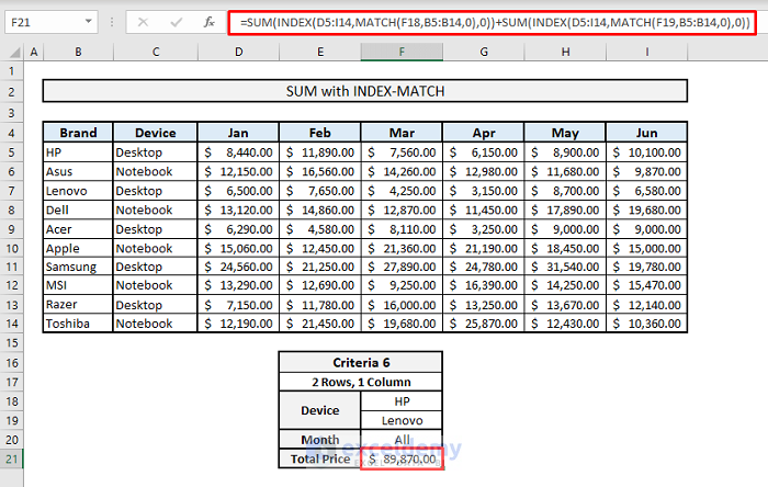
Criteria 6: Finding Results Based on 2 Rows and All Columns with SUM, INDEX, and MATCH Functions Together
Now let’s deal with 2 rows and all columns. We’ll find out the total selling prices for HP and Lenovo devices across all months.
Steps:
- In cell F21, use the following formula:
=SUM(INDEX(D5:I14,MATCH(F18,B5:B14,0),0))+SUM(INDEX(D5:I14,MATCH(F19,B5:B14,0),0))
- Press Enter, and you’ll find the resultant value as $89,870.
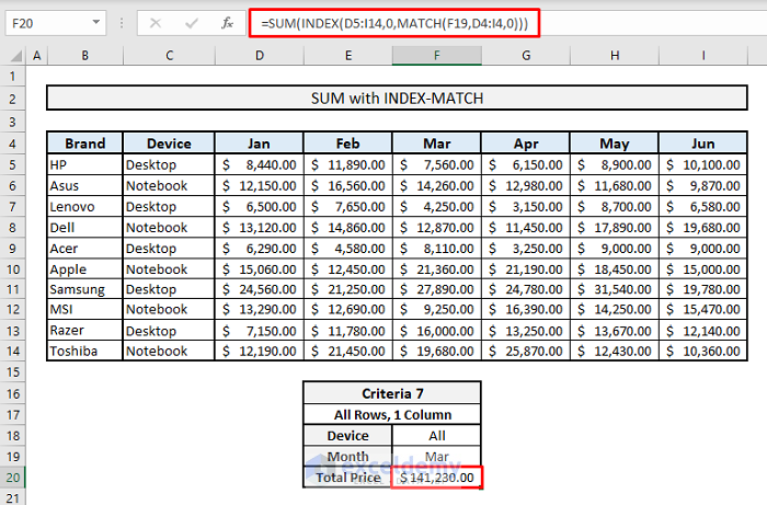
Criteria 7: Determining Output Based on All Rows and 1 Column with SUM, INDEX, and MATCH Functions Together
Under this criterion, we can extract the total selling prices of all devices for a single month (March).
Steps:
- In cell F20, type the following formula:
=SUM(INDEX(D5:I14,0,MATCH(F19,D4:I4,0)))
- Press Enter, and the return value will be $141,230.00.
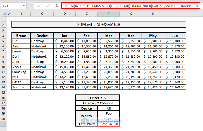
Criteria 8: Extracting Values Based on All Rows and 2 Columns with SUM, INDEX, and MATCH Functions Together
Now let’s determine the total selling price of all devices for two months: February and June.
Steps:
- In cell F21, use the following formula:
=SUM(INDEX(D5:I14,0,MATCH(F19,D4:I4,0)))+SUM(INDEX(D5:I14,0,MATCH(F20,D4:I4,0)))
- After pressing Enter, the total selling price will appear as $263,140.00.
Criteria 9: Finding Results Based on All Rows and All Columns with SUM, INDEX, and MATCH Functions Together
Let’s find out the total selling price of all devices for all months in the table.
Steps:
- In cell F20, type the following formula:
=SUM(INDEX(D5:I14,0,0))
- Press Enter, and you’ll get the resultant value as $808,090.00.
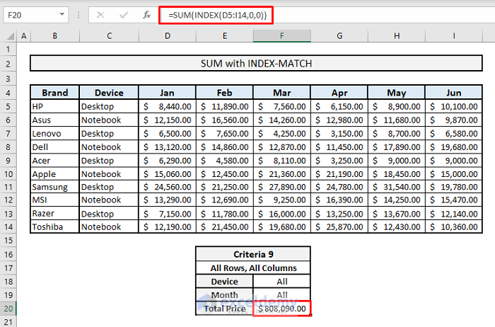
You don’t need to use MATCH functions here, as we’re defining all column and row positions by typing 0 inside the INDEX function.
Criteria 10: Calculating Sum Based on Distinct Pairs with SUM, INDEX, and MATCH Functions Together
In our final criterion, we’ll find out the total selling prices of HP devices for April along with Lenovo devices for June.
Steps:
- In cell F22, use the following formula:
=SUM(INDEX(D5:I14,MATCH({"HP","Lenovo"},B5:B14,0),MATCH({"Apr","Jun"},D4:I4,0)))
- Press Enter, and you’ll see the result as $12,730.00.
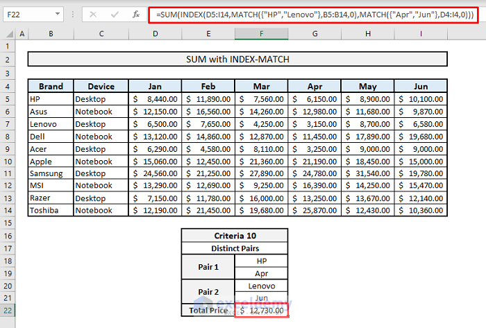
When adding distinct pairs in this combined function, insert the device and month names inside the two arrays based on the arguments for row and column positions, ensuring that the device and month names from the pairs are maintained in corresponding order.
Using SUMIF with INDEX-MATCH Functions to Sum Under Multiple Criteria
Before diving into the applications of another combined formula, let’s first introduce the SUMIF function.
- Formula Objective:
- The SUMIF function adds up the cells that meet specific conditions or criteria.
- Formula Syntax:
- =SUMIF(range, criteria, [sum_range])
- Arguments:
- range- Range of cells where the criteria lie.
- criteria- Selected criteria for the range.
- sum_range- Range of cells that are considered for summing up.
- Example:
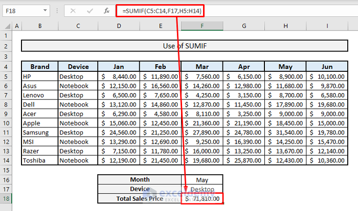
- Let’s use our previous dataset. Using the SUMIF function, we’ll find the total sales in May for desktops across all brands. The formula in cell F18 will be:
=SUMIF(C5:C14,F17,H5:H14)
- After pressing Enter, you’ll get the total sales price as $71,810.
- Let’s use our previous dataset. Using the SUMIF function, we’ll find the total sales in May for desktops across all brands. The formula in cell F18 will be:
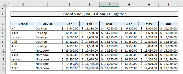
Now, let’s explore using SUMIF with INDEX & MATCH functions to sum under multiple criteria, considering both columns and rows. Our dataset has been slightly modified. In Column A, five brands are now present with multiple appearances for their two types of devices. The sales prices in the remaining columns remain unchanged.
Scenario:
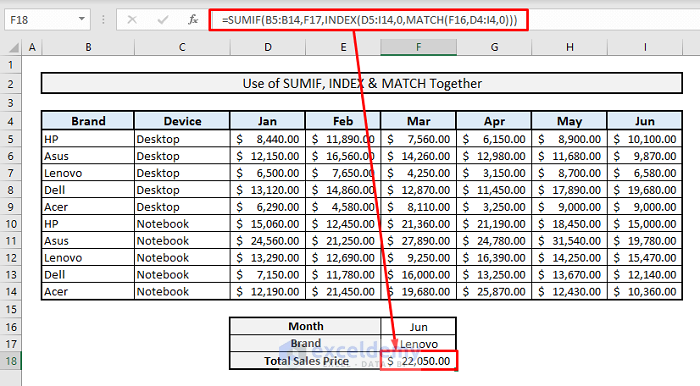
- We want to find out the total sales of Lenovo devices in June.
Steps:
-
- In the output cell F18, the related formula will be:
=SUMIF(B5:B14,F17,INDEX(D5:I14,0,MATCH(F16,D4:I4,0)))
- Press Enter, and you’ll get the total sales price for Lenovo in June.
- In the output cell F18, the related formula will be:
If you want to switch to the device category (assuming you want to find the total sales price for desktops), the Sum Range will be C5:C14, and the Sum Criteria will be “Desktop.” In that case, the formula will be:
=SUMIF(C5:C14,F17,INDEX(D5:I14,0,MATCH(F16,D4:I4,0)))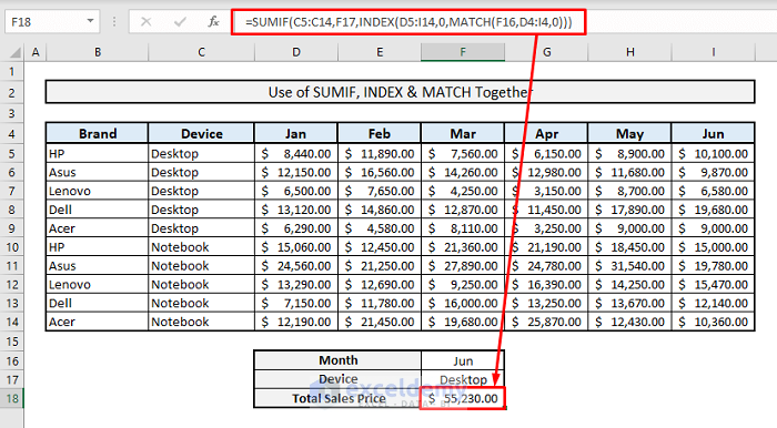
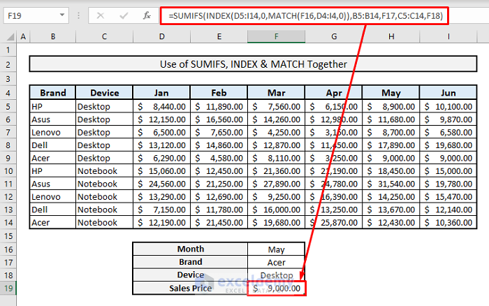
Using SUMIFS with INDEX & MATCH Functions in Excel
SUMIFS is a subcategory of the SUMIF function. By combining SUMIFS with INDEX & MATCH functions, you can add more than one criterion, which is not possible with SUMIF alone. In SUMIFS, you input the Sum Range first, followed by the Criteria Range and the range criteria.
Scenario:
- Let’s find out the sales price of Acer desktops in May. Along the rows, we’re adding two different criteria from Columns B & C.
Steps:
- The related formula in cell F19 will be:
=SUMIFS(INDEX(D5:I14,0,MATCH(F16,D4:I4,0)),B5:B14,F17,C5:C14,F18)
- Press Enter, and the function will return $9,000.00.
Download Practice Workbook
You can download the practice workbook from here:
<< Go Back to Multiple Criteria | INDEX MATCH | Formula List | Learn Excel
Get FREE Advanced Excel Exercises with Solutions!

I recreated the table/data you are using as your example but while attempting to use “Use of SUMIFS with INDEX & MATCH Functions in Excel” formula (=SUMIFS(INDEX(D5:I14,0,MATCH(F16,D4:I4,0)),B5:B14,F17,C5:C14,F18)), it keeps returning a “#N/A” with the message, “Error Argument must be a range.”
Any idea where I’m going wrong?
The formula is working at our end perfectly. You can download the workbook where we did the whole thing and cross-check, please.
Extracting data based on one Row and Two Columns:Using the downloaded work book, I evaluated the look up value {“Feb”,”Jun”} in the match function and returned 2 as the column position. The returned value was the selling price for only Feb and yet we were looking at 2 columns (Feb and Jun)
Please re-check and advise
Hello Peter and Charlie, the solution described in this article at Criteria 2: “Extracting Data Based on 1 Row & 2 Columns with SUM, INDEX and MATCH Functions Together” is perfectly working from our end.
Just to inform you, you can’t use a cell reference in the Look_up value of the MATCH function instead you have to insert the single of multiple look_up values manually e.g. {“Feb”,”Jun”}. Hope you have found your solution. Try it and let us know the outcome in a reply. Thank you!
I’m running into the same problem. I can’t look up multiple criteria using MATCH in the same row. It only returns one of the values.
Do you have examples where there are two criteria along the top, ex month & year, and in some situations you need full year and in others you need only last month? Thank you
Hello ALLISON!
you can use the “Use of SUMIF with INDEX-MATCH Functions to Sum under Multiple Criteria” method for your problem. Here, we have used the brand name as criteria and you can substitute it by Year. See this screenshot below:
While using this method, you have to fill in both criteria. So, you must put both the year’s and month’s values.
I hope, your problem will be solved in this way. You can share more problems in an email at [email protected]
What if I wanted to sum the value of all Lenovos and all desktops in the month of June without double-counting the Lenovo desktop sold in that month? The total should be 70,700, but if I add the total of all Lenovos for the month of June and all desktops for the month of June, it ends up as 77,280 (this is taken from the table in the second, third, and fourth screenshots of the section entitled ‘Use of SUMIF with INDEX-MATCH Functions to Sum under Multiple Criteria’), because the Lenovo desktop in June (6,580) gets counted twice. How can we avoid this double-counting and use a formula that would arrive at the total of 70,700 (and could it be used if there was a third criterion–OR not AND–that we wanted to sum without double and triple counting the instances where more than one of these criteria was met)?
Hello, JOHN!
Thanks for your comment!
I’m not sure about your problem, you want all Lenovos that means the Desktop and Notebook! Also, All the desktops that mean the range of C5:C9!
Can you please send me your excel file via email? ([email protected]).
You can use this https://www.exceldemy.com/sum-index-match-multiple-criteria-in-excel/#Use_of_SUMIFS_with_INDEX_MATCH_Functions_in_Excel
This may fulfill your criteria.
Good Luck!
Regards,
Sabrina Ayon
Author, ExcelDemy.
What if I wanted to do QTD numbers by brand?
How do I get QTD by brand?
Dear ALEX,
Thank you for this interesting question. If you want to find the total sales value for each brand within a quarter or QTD, you can use a formula that combines the SUMIFS, INDEX, and MATCH functions.
Formula:
=SUMIFS(INDEX(D5:I14,0,MATCH(D16,D4:I4,0)),B5:B14,D17,C5:C14,D18)+SUMIFS(INDEX(D5:I14,0,MATCH(E16,D4:I4,0)),B5:B14,D17,C5:C14,D18)+SUMIFS(INDEX(D5:I14,0,MATCH(F16,D4:I4,0)),B5:B14,D17,C5:C14,D18)The formula used here is the same as the one explained in the “Use of SUMIFS with INDEX & MATCH Functions in Excel” section. We repeat the formula two more times, adjusting the column reference for each specific month in the quarter.
I hope this solution resolves your issue. Feel free to email us at [email protected] if you have any further problems or inquiries.
Regards,
Qayem Ishrak Khan
Team ExcelDemy.
Hello,
Can you help me with below
=IFNA(INDEX($G$20:$G$52,MATCH(1,($B$20:$B$53=$B3)*($E$20:$E$52=$D3)*($F$20:$F$52=CH$1)*($A$20:$A$53=$A3)*($D$20:$D$52=$E3),0)),”0″)
this formula returns value based on multiple matches. But when i have more than one value, return is only 1st value. How can i change it to get all values sum instead.
Hello, RUSSEL.
Thank you for sharing your problem with us. We have provided 2 different ways to solve your problem.
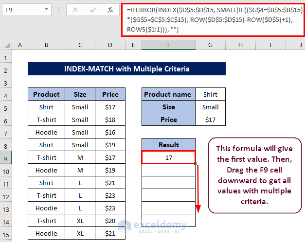
For example, we have a dataset of Product, Size, and Price. We will find the total price of the Small Shirts.
Method-1:
For this, write the following formula in the F9 cell and press Enter.
=IFERROR(INDEX($D$5:$D$15, SMALL(IF(($G$4=$B$5:$B$15)*($G$5=$C$5:$C$15), ROW($D$5:$D$15)-ROW($D$5)+1), ROWS($1:1))), "")And, you will get the first Price value.
Then Drag the F9 formula downwards to get other Price values that meet the criteria.
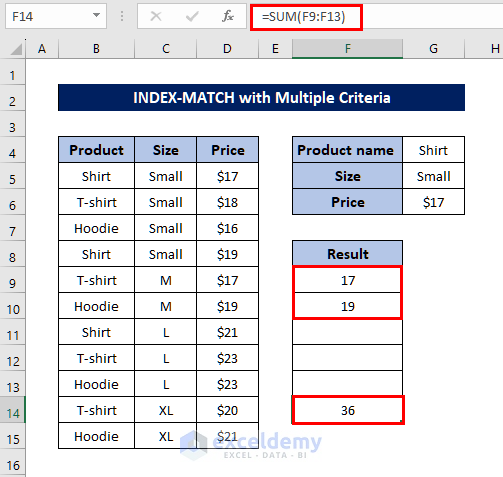
You can see that we have got two Price values that meet the multiple criteria.
Now, you can use the SUM function to get the total Price value.
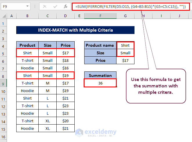
Method 2:
Write the following formula in F9 and press Enter.
=SUM(IFERROR(FILTER(D5:D15, (G4=B5:B15)*(G5=C5:C15)), ""))And, you will get the total Price value with multiple criteria.
The FILTER function used in this method is only available for Microsoft 365 and Excel 2021.
Solution to Your Problem:
You can use the formula below to solve your problem:
=SUM(IFERROR(FILTER($G$20:$G$52, ($B$20:$B$53=$B3)*($E$20:$E$52=$D3)*($F$20:$F$52=CH$1)*($A$20:$A$53=$A3)*($D$20:$D$52=$E3)), ""))We could have given you the exact formula if we had your dataset. Let us know if your problem is solved.
Regards,
Sourav
ExcelDemy.