Spreadsheets are used in many jobs to keep track of, organize, and look at data. By adding column headers to your data in Excel, you can organize it and make it easier to read. This article talks about how to create column headers in Excel and why it’s important to do so in three different ways.
How to Create Column Headers in Excel: 3 Methods
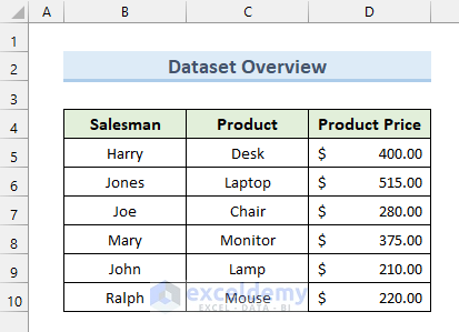
There are three ways to create column headers in Excel. See the table in the next example for a good way to explain these procedures and how they work. It shows how a company is going to sell certain products.
The three different methods and their steps are given below.
1. Creating Column Headers by Freezing a Row
Use these three steps to create column headers in Excel by freezing a row.
Steps:
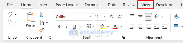
- First, click the View tab.
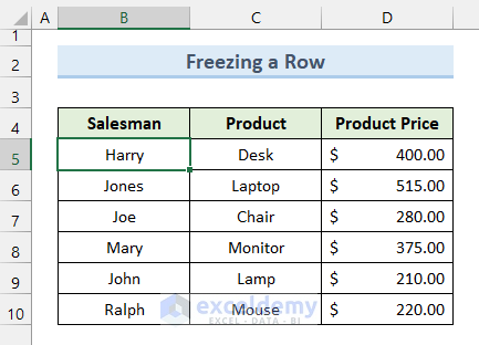
- Second, choose the frame right inside the row and column we need to create headers. To do this, select the corner cell of the area that we want to keep unlocked. In our case, we will select the cell Harry to freeze the upper panes.
- Third, in the View tab, choose Freeze Panes option.

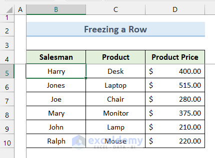
- As a result, this will freeze the rows above the selected cell and the columns.
Read More: How to Change Column Headings in Excel
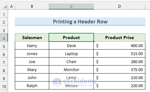
2. Printing a Header Row to Create Column Headers
If we want to repeat column headings on each page throughout all the Excel sheets, we can follow this method. Here’s a list of five steps to creating a header row by printing in Excel.
Steps:
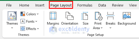
- Firstly, select the Page Layout tab.
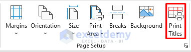
- Secondly, click the Print Titles.
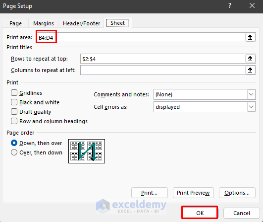
- Thirdly, make sure that the cells in which the data is included are selected as the Print Area. After clicking the button that is located next to the Print Area box, move the selection so that it covers the data that you want to print.
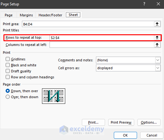
- Next, click on Rows to repeat at top. This will let you choose which row(s) to treat as the constant header.
- Then, choose the row(s) you wish to make a header for. The rows you choose will be at the top of every printed page. This is particularly useful for making huge spreadsheets accessible over numerous pages.
- In addition, click the button next to Columns to repeat at left. This will allow you to select columns that you want to keep constant on each page.
- Lastly, we can print the sheet. Excel will use the constant heading and the columns you selected in the Print Titles box to print the data that you specified.
Read More: How to Remove Column Headers in Excel
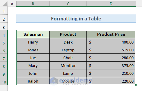
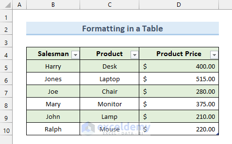
3. Creating Column Headers by Formatting in a Table
The Excel Table can generate row or column headers automatically when you transform your data into a table.
Steps:
- At first, choose the information you want to put into a table.
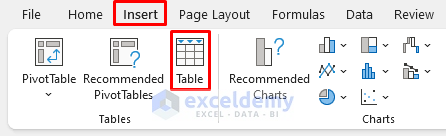
- Then click the Insert tab and select the Table option.
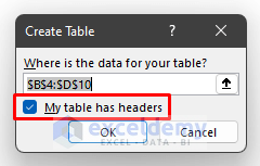
- Next tick the My table has headers box and then click OK. The first row will automatically become column headers.
- In the end, we will get a table like the image below.
Read More: How to Rename Column in Excel
Things to Remember
- Format column heads differently and use Freeze Panes to always see them. It saves time by reducing scrolling.
- Print using Print Area and Rows to repeat at every page.
- Excel Tables need definite range and column headings.
Download Practice Workbook
You can download the practice workbook from here.
Conclusion
Creating column headers in Excel is an important thing that might help us while making big data sheets. Hope this article helped with that purpose. If you’re still having trouble with any of these methods, let us know in the comments. Our team is ready to answer all of your questions.
Related Articles
- How to Remove Column1 and Column2 in Excel
- How to Title a Column in Excel
- How to Change Excel Column Name from Number to Alphabet
- How to Change Column Header Name in Excel VBA
- [Fixed] Excel Column Numbers Instead of Letters
<< Go Back to Rows and Columns Headings | Rows and Columns in Excel | Learn Excel
Get FREE Advanced Excel Exercises with Solutions!
