
In Excel, you can build regression models easily without any complex coding. In this tutorial, we show 7 steps to building a regression model in Excel.
Assume you’re analyzing how Advertising Budget affects Sales (and possibly other factors like Price and Online Reach).
Step 1: Organizing Your Data
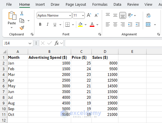
- Open Excel and input your data in a worksheet. Organize it with independent variables (predictors) in one or more columns and the dependent variable (outcome) in another.
- Independent variable(s): Advertising, Price
- Dependent variable: Sales
- Avoid blank rows or merged cells
- Ensure numerical columns are formatted correctly
Step 2: Creating a Scatter Plot
A scatter plot helps visualize the relationship between two variables.
Steps:
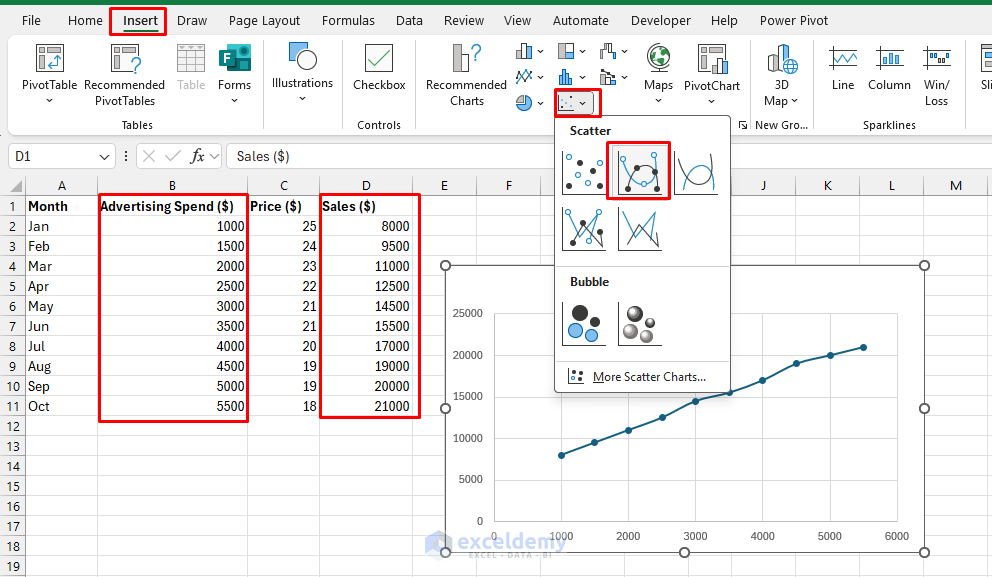
- Select your data.
- Independent variable (Advertising Spend)
- Dependent variable (Sales)
- Go to the Insert tab >> from Charts >> select Scatter >> select Scatter with Smooth Line and Markers
- Add titles:
- Chart title: Advertising Spend vs. Sales
- X-axis: Advertising Spend
- Y-axis: Sales
- You’ll see points showing how Sales respond to Advertising spending
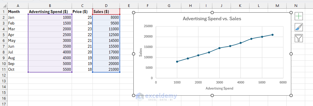
Interpretation: If the points rise from left to right, there’s a positive correlation (higher advertising → higher sales).
Step 3: Adding a Trendline
To visualize the linear relationship directly:
- Click on a data point in the scatterplot
- Choose Add Trendline >> select Linear >> select More Options
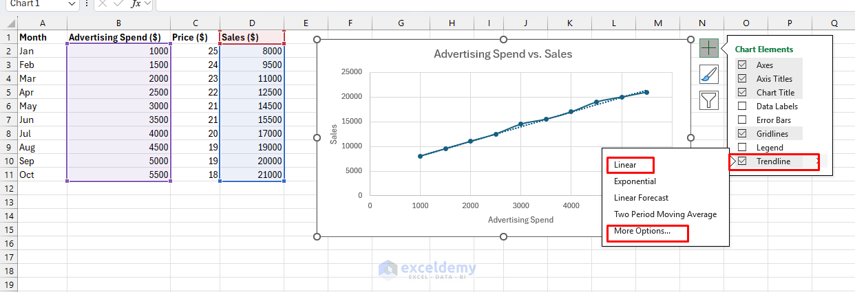
- Check the boxes for:
- Display Equation on chart
- Display R-squared value on chart
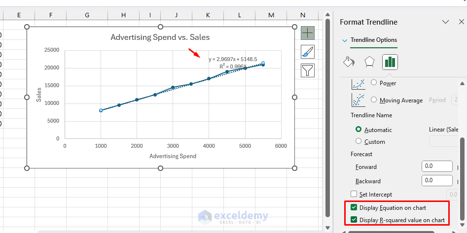
Output:

y = 2.9697x + 5148.5
R² = 0.9961
Here:
- y = Sales
- x = Advertising Spend
- For every $1,000 increase in advertising, sales increase by about $2,969.70
- R² = 0.9961 means 99% of the variation in Sales is explained by Advertising Spend
Step 4: Understanding the LINEST Function for the Regression Model
The LINEST function provides detailed regression statistics beyond what a trendline shows. It computes precise coefficients and statistics directly in worksheet cells.
Syntax:
=LINEST(known_y's, known_x's, [const], [stats])
Parameters:
- known_y’s: Your dependent variable (Sales)
- known_x’s: Your independent variable(s) (Advertising Spend, etc.)
- const: TRUE (include intercept) or FALSE
- stats: TRUE (return full statistics) or FALSE
Use LINEST to:
- Get precise coefficients for predictions
- Assess statistical significance
- Handle multiple predictor variables
- Calculate standard errors and confidence intervals
Step 5: Running Simple Linear Regression with LINEST
Build a simple linear regression model in Excel using Advertising Spend to predict Sales.
Steps:
- Select a blank 5-rows × 2-columns range (for example, F2:G6) to capture the full statistics output
- Enter the following formula
=LINEST(D2:D13, B2:B13, TRUE, TRUE)
Where:
- D2:D13 → Sales
- B2:B13 → Advertising
Output (5×2 array): Advertising Spend vs. Sales

- Row 1 – Coefficients:
- Slope: 2.97
- Intercept: 5148.49
- Equation:
Sales = 2.97 × Advertising Spend + 5148.49
-
- Business insight:
- For every $1 increase in advertising, sales increase by about $2.97
- With zero advertising, you’d have base sales of about $5,148.49
- ROI: Roughly a 3× return on advertising investment (in this sample)
- Business insight:
- Row 2 – Standard errors
- Slope SE: 0.065
- Intercept SE: 232.43
- These are small relative to the coefficients, indicating reliable estimates
- Row 3 – Model quality
- R²: 0.996 = 99.6%
- Standard error of the regression: 297.08
- Interpretation:
- Exceptional fit. About 99.6% of sales variation is explained by advertising spend
- Predictions are typically off by ±$297 (given sales range from roughly $8,000–$21,000)
- Row 4 – Statistical significance
- F-statistic: 2060.94 (extremely high)
- Degrees of freedom: 8
- The very high F-statistic indicates a highly statistically significant relationship
- Row 5 – Variance breakdown
- Regression SS: 181,893,939
- Residual SS: 706,060
The regression sum of squares is much larger than the residual sum of squares, confirming excellent model fit.
Step 6: Running Multiple Linear Regression with LINEST
Now build a multiple linear regression model using multiple independent variables (Advertising Spend + Price) for better predictions.
Steps:
- Select a 5-rows × 3-columns cell range (for full statistics output; for example, F2:H6)
- Enter the following formula
- If you are using an older version of Excel, press Ctrl + Shift + Enter
=LINEST(D2:D13, B2:C13, TRUE, TRUE)
- D2:D13 → Sales
- B2:C13 → Advertising and Price
This model includes both Advertising Spend and Price as predictors.
Output (5×3 array): Advertising + Price vs. Sales

- Row 1 – Coefficients appear in REVERSE order (read right to left):
- Intercept: 19133.73
- Advertising coefficient: 2.16
- Price coefficient: -536.15
- Equation:
Sales = 2.16 × Advertising Spend - 536.15 × Price + 19133.73
-
- Business insight:
- Each $1 in advertising → about $2.16 increase in sales (holding Price constant)
- Each $1 increase in price → about $536 decrease in sales (holding Advertising constant)
- Price has a strong negative impact on sales, as expected
- Business insight:
- Row 2 – Standard errors
- Price SE: 243.30
- Advertising SE: 0.37
- Intercept SE: 6349.25
- Both predictors are reasonably precise (errors are small relative to coefficients)
- Row 3 – Model quality
- R²: 0.997 = 99.7%
- Standard error of the regression: 244.04
- Interpretation:
- Slightly better than simple regression (99.7% vs. 99.6%)
- Adding Price improves the model marginally
- Prediction error reduced to about ±$244 (from ±$297)
- Rows 4–5
- F-statistic: 1529.60 (very high)
- Degrees of freedom: 7
- The model is statistically robust
Interpreting the Results
Key Comparisons:
| Metric | Simple Regression | Multiple Regression |
|---|---|---|
| R² | 99.6% | 99.7% |
| Standard Error | $297 | $244 |
| Predictors | Advertising only | Advertising + Price |
Business Insights:
- Both models perform excellently
- Advertising is highly effective: Strong positive relationship with sales in both models
- Price matters: The multiple regression shows that each $1 price increase is associated with about a $536 decrease in sales. Adding Price gives slightly better predictions (lower error).
- Consider pricing strategy carefully
- Lower prices may boost sales significantly
- Predictive power: With R² ≈ 99.7%, you can forecast sales very accurately using:
- Planned advertising budget
- Intended pricing

Step 7: Running Regression Using the Data Analysis ToolPak
You can use the Data Analysis ToolPak to get detailed output (coefficients, R², significance). It provides a comprehensive report with detailed statistics.
Enable Data Analysis ToolPak:
- Go to File >> Options >> Add-ins >> Excel Add-ins >> click Go
- Check Analysis ToolPak >> click OK
Steps:
- Go to the Data tab >> select Data Analysis >> select Regression >> click OK

- Set Regression:
- Input Y Range: Select Sales data, including headers (dependent variable)
- Input X Range: Select Advertising Spend, including headers (or multiple independent variables)
- Check Labels
- Choose an Output option: New Worksheet Ply

Output:

Interpretation:
- Intercept: 5148.48
- Advertising Spend ($): 2.9697
- R²: 0.9961
- P-values: Intercept = 1.82E-08, Advertising = 6.12E-11
- Standard error of the regression: 297.08
Advertising strongly and reliably increases Sales in this dataset, and the linear model explains almost all of the variation.
Both approaches (formula and Data Analysis) fit the same linear model. Coefficients, R², F/df, and (when computed) p-values match.
When to Use LINEST vs. Data Analysis → Regression
Use the LINEST function when:
- You want live, formula-driven results that recalculate with the data (great for what-if dashboards)
- You want to reference coefficients in other formulas (predictions, scenarios)
- You’re comfortable with array outputs and, if needed, computing p-values from t = β/SE
Use Data Analysis → Regression when:
- You want a readable, one-click report with p-values and confidence intervals shown directly
- You’re teaching/reporting and need a formatted ANOVA table
- You don’t need results to update automatically when data change
Bonus: Predicting Future Sales
Once you have your regression equation, you can predict future sales.
Assume you plan to spend $6,000 on advertising and set the price at $17. Predict sales with the multiple regression model.
Using Multiple Regression:
Sales = 2.16 × Advertising Spend - 536.15 × Price + 19133.73
= 2.16 * 6000 - 536.15 * 17 + 19133.73
= 22979.18
Your model predicts approximately $22,979 in sales for this scenario.
Download Practice Workbook
Conclusion
You can follow these 7 steps to build a regression model in Excel. Excel provides essential tools for regression analysis, including scatterplots, Trendlines, the Data Analysis ToolPak, and the LINEST function. With these, you can identify relationships between variables, quantify trends with coefficients, and predict future outcomes. Whether it’s sales forecasting, cost prediction, or performance analysis, regression in Excel is a powerful and accessible method for turning your data into insights.
Get FREE Advanced Excel Exercises with Solutions!
