What Is a 3D Reference in Excel (With 2 Suitable Uses)

This tutorial explains what a 3D reference is in excel and how we can use it. We will also learn how we can create a 3D formula to cluster data in various worksheets. Excel’s 3D reference is also known as a dimensional reference which is one of excel’s greatest cell reference attributes. In this article, we will give 2 examples of using a 3D reference in excel to clarify the concept to you.

Download Practice Workbook

You can download the practice workbook from here.

What Is a 3D Reference in Excel?

The same cell or set of cells on numerous worksheets is referred to as a 3D reference in Excel. It’s a simple and quick approach to combining data from multiple worksheets with the same structure. We can use 3D reference in excel instead of Excel’s Consolidate feature.

Generate a 3D Reference in Excel

To generate a 3D reference in excel across multiple worksheets, we will use a generic formula. The formula is given below:

or,

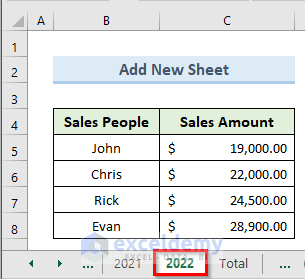
To illustrate the examples of this article we will apply the above formulas in the following dataset. From the dataset, we can see that we have sales data of different salespeople for 3 years 2019, 2020, and 2021 respectively.

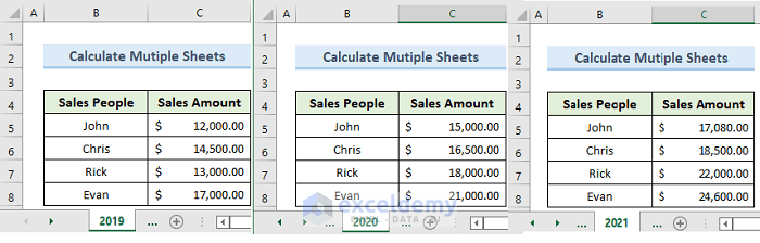
We will use a 3D Reference formula to calculate the total sales amount in 3 years for each salesperson in another sheet named Total.

2 Suitable Uses of 3D Reference in Excel

1. Calculate Total from Multiple Sheets Using 3D Reference in Excel

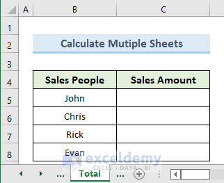
In the first example, we will see how we can calculate the total amount of sales for 3 years in a new sheet named Total. To perform this method we will follow the below steps.

STEPS:

• To begin with, go to the sheet named Total.
• In addition, select cell C5.
• Furthermore, type the following formula in that cell:

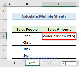
• Now, press Enter.
• So, in cell C5 we get the total value of cell C5 from all the worksheets between 2019 to 2021.
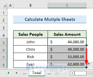
• After that, drag the Fill Handle tool from cell C5 to C8.
• Lastly, we get results like the following image.

Read More: How to Use SUM and 3D Reference in Excel (Detailed Analysis)

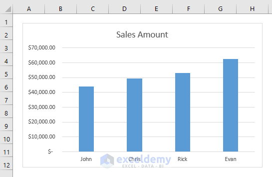
2. Use 3D Reference to Create a Chart

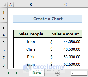
In the second method, we will see how we can create a chart in excel using a 3D reference. In the following image, we have a dataset of sales data. Using this dataset as a reference we will create a chart in a different worksheet.

Let’s see the steps to make a chart using reference.

STEPS:

• Firstly, open a new blank sheet named Chart.
• Secondly, go to the Insert tab.
• Thirdly, click on the dropdown ‘Insert Column or Bar Chart’.
• Then, from the dropdown menu select a bar chart option

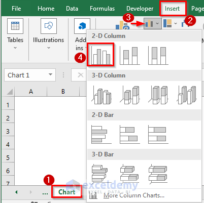
• So, the above action returns a blank chart.
• Afterward, right-click on the blank chart and click on the option Select Data.

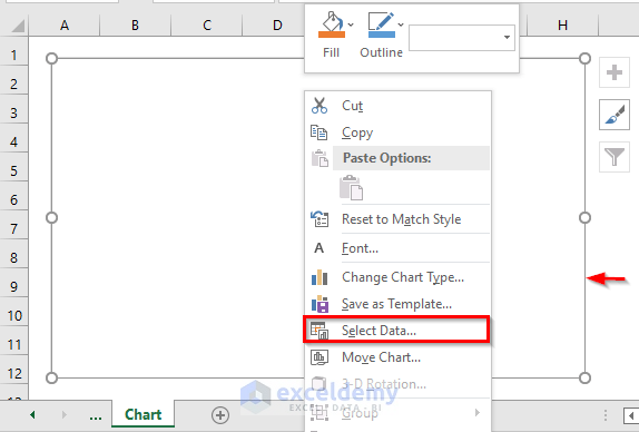
• Moreover, the above action opens a new dialogue box named ‘Select Data Source’.
• After that, go to the source worksheet sheet named Data. Select cell range (B4:C8) from that worksheet.
• Now, click on OK.

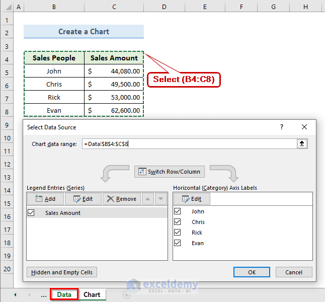
• Finally, we can see our desired chart in the following image.

Read More: 3D Referencing & External Reference in Excel

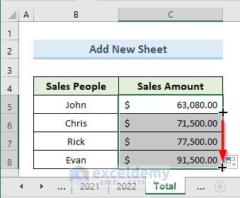
Add a New Excel Sheet in Current 3D Cell Reference

Until now we know a 3D reference in excel encapsulates multiple worksheets at the same time. What if we want to add a new excel sheet to our existing reference. In this section, we will discuss how we can add an excel sheet to our existing cell reference. Follow the below steps to perform this method.

STEPS:

• First, add a new sheet to the end of the last sheet.

• Next, go to the sheet Total.
• Then, select cell C5. Modify the previous formula like the following one:

• Now, press Enter.
• As a result, in cell C5 we can see the total value of cell C5 from all the worksheets between 2019 to 2022.
• After that, drag the Fill Handle tool from cell C5 to C8.
• Finally, we get results like the following image.

NOTE:

• If we add a sheet to the first point then we have to modify the first argument of the reference formula.
• The reference formula will update automatically if we add or delete any sheet in between the two reference sheets.

Things to Remember

• We have to use the same type of data in all worksheets.
• If the worksheet is moved or removed, Excel can still link to the precise cell range.
• The result will also change if we add any worksheet between the referencing worksheet.

Conclusion

In conclusion, from this tutorial, we get to know what a 3D reference is in Excel. To put your skills to the test, download the practice worksheet included in this article. Please leave a comment in the box below if you have any questions. Our team will try to react to your message as quickly as possible. In the future, keep an eye out for more innovative Microsoft Excel solutions.

Related Articles

• 3D Reference Not Working in Excel (3 Reasons & Solutions)