How to Create a Chart from Selected Range in Excel – 4 Methods

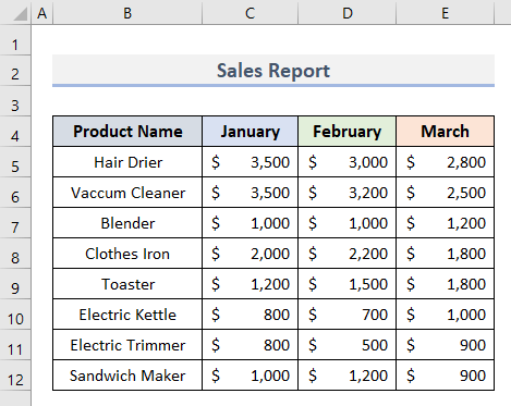
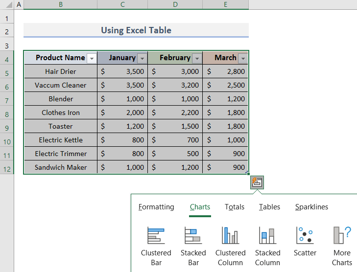
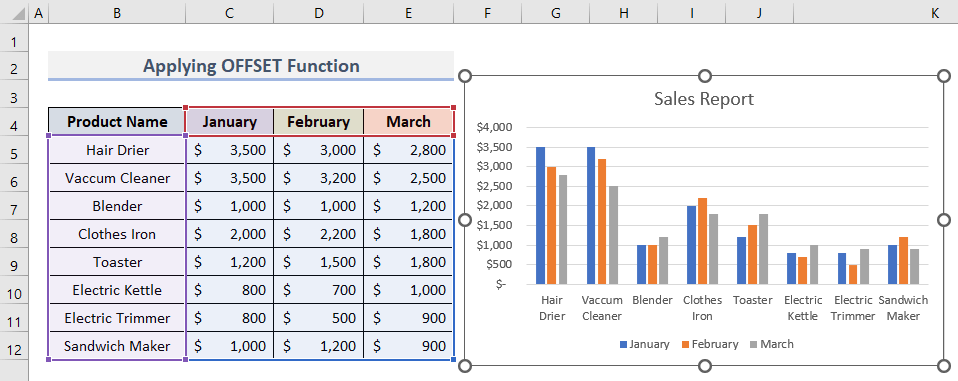
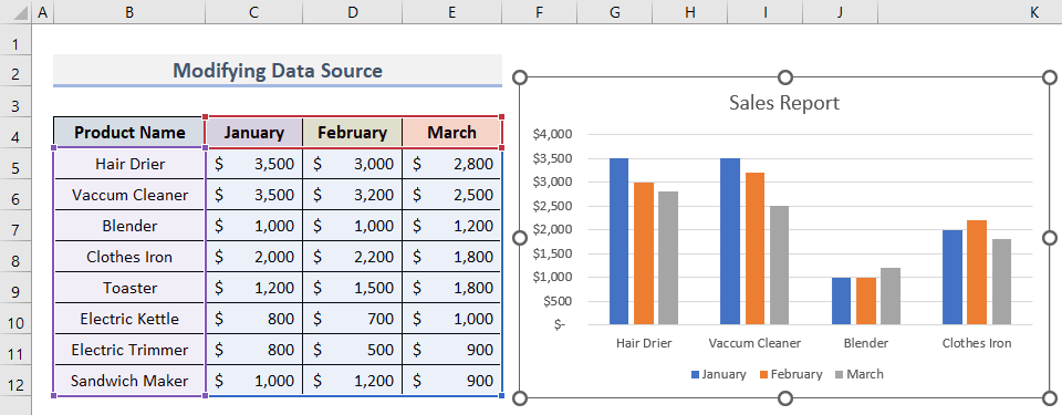
The dataset below showcases a Sales Report of electric products in January, February, and March.

Method 1 – Create a Chart from the Selected Range Using an Excel Table

Create a graph or chart from a Table:

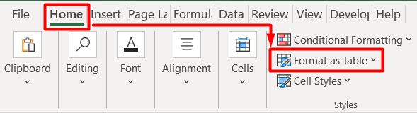
• Go to the Home tab and select Format as Table in Styles.

• Select all the cells in the table and left-click.

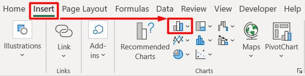
• In the Insert tab, select Bar Chart in Charts.

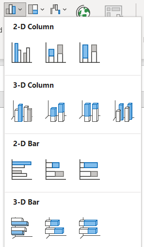
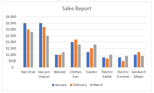
• Choose a chart.

• You can also select the range and right-click to select Quick Analysis and choose Charts.

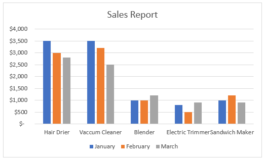
• The chart is displayed in your worksheet.

Read More: How to Make an X-Y Graph in Excel

Method 2 – Applying the OFFSET Function to Create a Chart from a Selected Cell Range

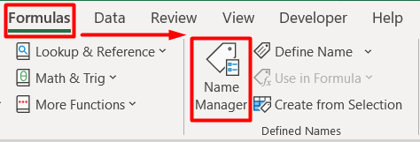
• Select Formulas and choose Defined Name in Name Manager.

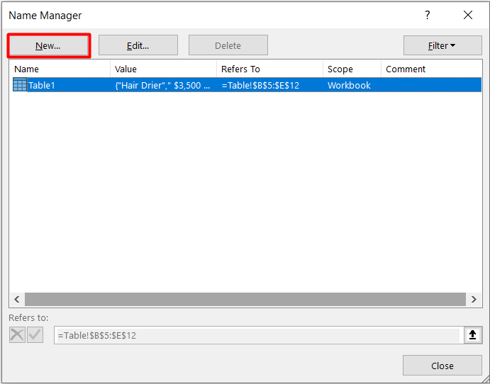
• In the dialog box, select New to create a new Name Range.

• Enter TableForChart in Name:.
• Enter this formula in Refers to:.

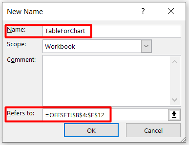
Using the OFFSET function, the chart will automatically update if data is changed.

• Click OK.

You will see the Name Range in the Name Box.

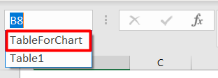
• Select the Name Range in the Name Box.
• Follow the same steps described in Method 1 to insert a chart..

Read More: How to Make a Graph in Excel That Updates Automatically

Method 3 – Modify the Data Source to Create a Chart from a Selected Range

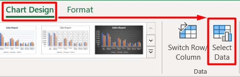
• Select the existing chart.
• Click Design to select Select Data in Data.

• In Horizontal (Category) Axis Labels, select the categories you want to display in the chart.

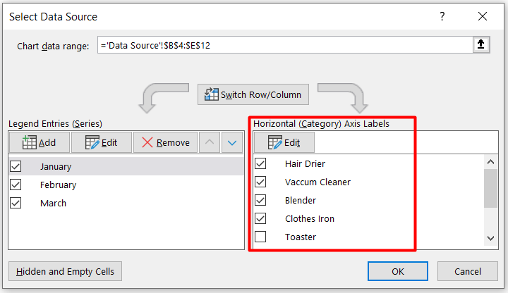
• Click OK.
• You will see a new chart in your worksheet:

Read More: How to Plot Graph in Excel with Multiple Y Axis

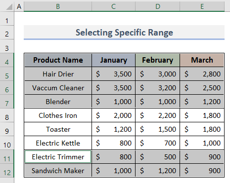
Method 4 – Select a Specific Range to Create a Chart in Excel

To create a chat with 5 products:

• Select the 5 products data: B4:E7 and B11:E12.

• Go to the Insert tab and click Recommended Charts.

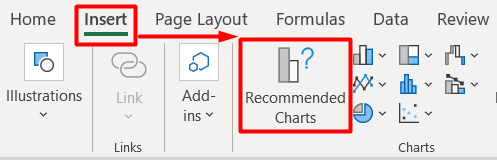
• Select any type of chart in All Charts.

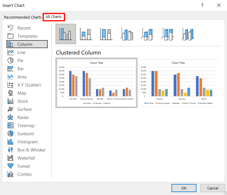
• Click OK.
• The cart will display the selected product information only.

Read More: How to Display Percentage in an Excel Graph

Things to Remember

• Press Ctrl + T to create a table from your dataset.
• When you add new data to the worksheet, the chart will automatically update  If you delete data, not all data points will be removed from the chart.
• Make sure there are no blank cells in the dataset.

Download Practice Workbook

Download the sample file.

<< Go Back To How to Create a Chart in Excel | Excel Charts | Learn Excel