How to Track Attendance in Excel (with Detailed Steps)

Elements of an Attendance Tracker

To make an attendance tracker in Excel, you will need the following:

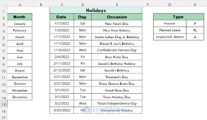
Month
Holidays
Types of Activity: P= Present, PL = Planned Leave, A= Absent
Days of Month, Start & End date of Month
Participant Name & Id
Total Present, Planned Leave, Absence & Workdays
Percentage of Presence & Absence

You can add or remove any columns as you need. We will make a template with the mentioned elements.

Step 1 – Making an ‘Information’ Worksheet in Excel

In this worksheet, add the lists of Months, Holidays, and the Type of activities that will be used to track attendance (present/absent or reason). You can also add the employee names and IDs to link to the main worksheet.

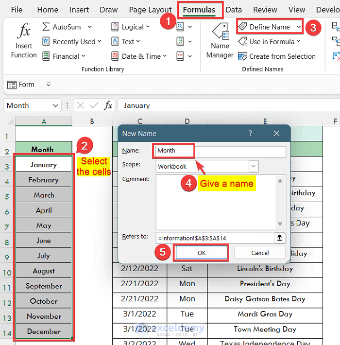
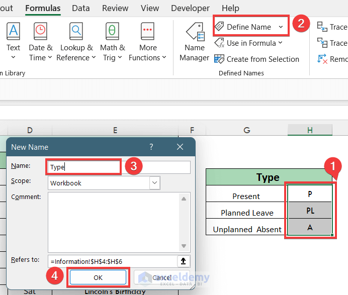
NOTES: We haven’t listed all the holidays in this workbook. You can add or remove holidays as per your company.

Step 2 – Defining the Name of the Month List

Select the cells of months.
Go to the Formula tab and click on the Defined Name option.
You will see a window named “New Name”. Insert a suitable name for the list of cells. We chose “Month” for the Name.
Press OK.

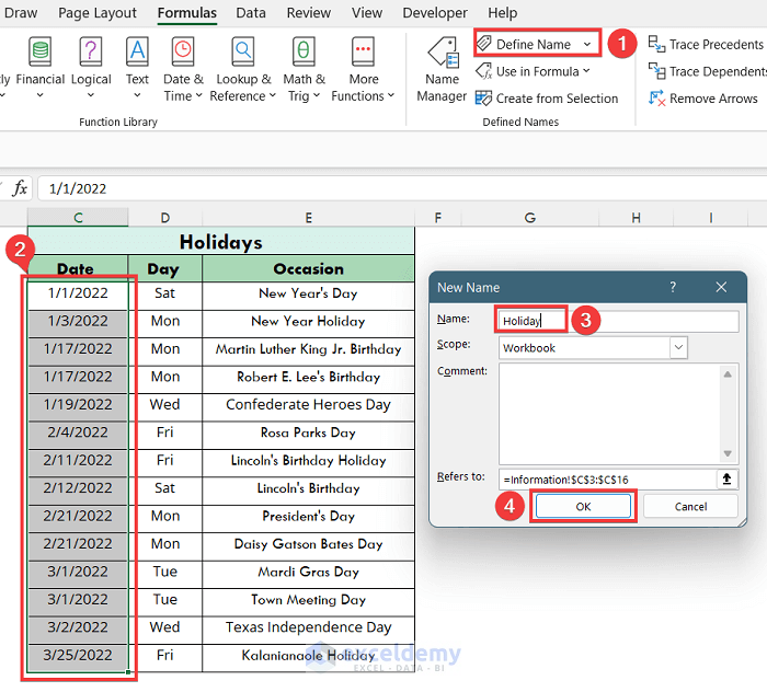
Select the holiday cells and go to the Defined Name option.
Type “Holiday” as the name and press OK.

Select the Type cells and go to the Defined Name option.
Put “Type” as the name and press OK.

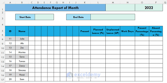
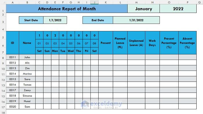
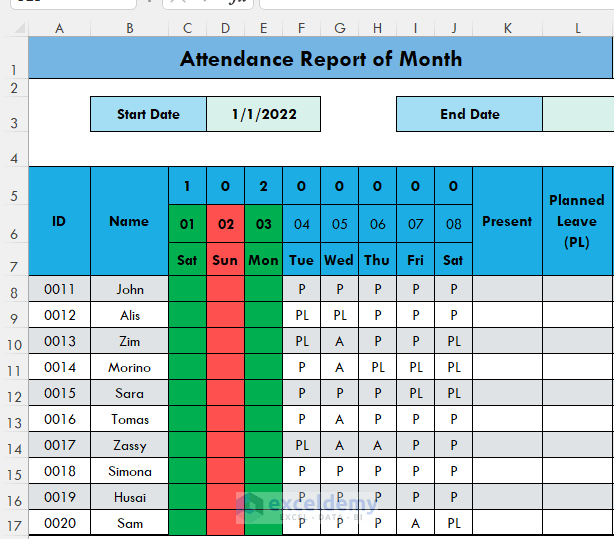
Step 3 – Making a Template Structure to Track Attendance

Make columns and cells with the necessary things listed before. Insert the data of employee or participant names and IDs.

Step 4 – Inserting Formula for Month, Start Date, and End Date

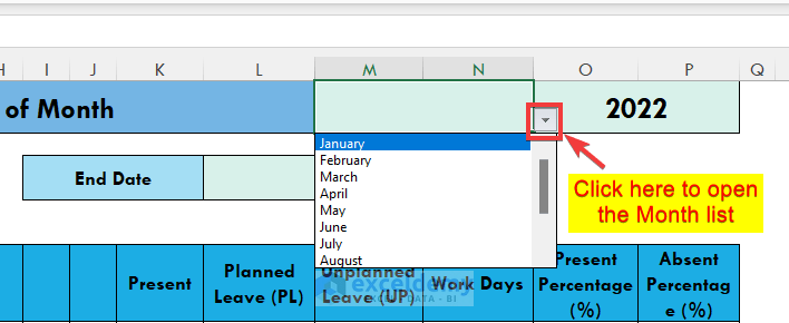
Select the month cell.
Go to the Data tab and click on the Data Validation option

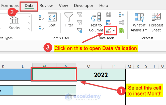
A window named “Data Validation” will appear.
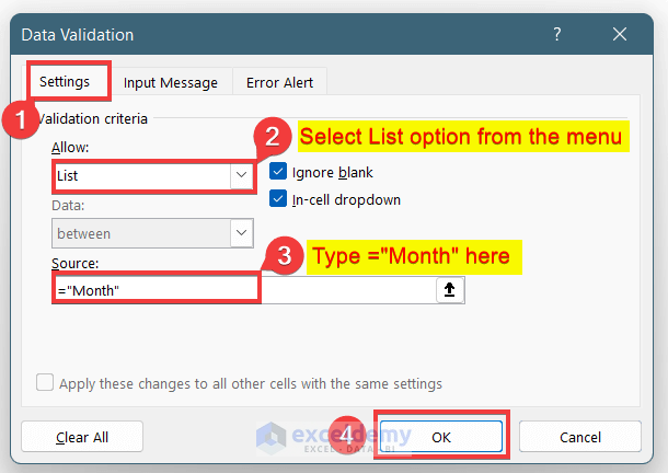
Select the “List” option in the Allow menu.
Type “=Month” in the Source option and press OK.

If you go to the month cell in the worksheet, you will see a drop-down.
Click on it and select a month.

Use this formula in the Start Date cell.

=DATEVALUE("1"&M1)

Formula Explanation :

DATEVALUE function transforms a date that is in Text format into a valid Excel date
Here, the M1 cell is the month cell giving value “January”
“1”& “January” denotes a date “1st January”

Insert this formula in the End Date cell to get the last date of the month.

=EOMONTH(D3,0)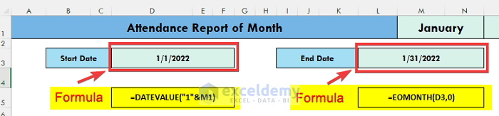

Step 5 – Entering the Dates

Enter the first date of the month. Use formula to link the cell with the Start Date cell:

=D3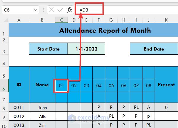

Make a column for the remaining dates.
In the second cell, use this formula to get the next date.

=IF(C6<$L$3,C6+1,"")

Formula Explanation:

C6<$L$3 : Denotes a condition that cell C6 (Previous Date before this cell) is less than L3 (End Date). You must use absolute reference because the cell of End Date will be the same for the next cells also.
C6 + 1 : Adds 1 with the previous cell.
“” : If the “If” returns False, keep the cell blank.

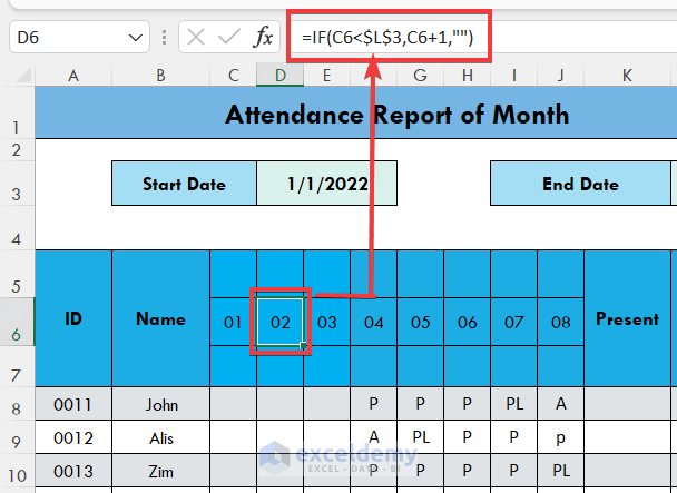
Drag the formula through the row.

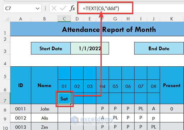
Paste this formula into cell C7:

=TEXT(C6, "ddd")

Formula Explanation:

The TEXT function will convert the Date value of the C6 cell to text.
“ddd” denotes the format of the text which will give the name of the weekday in 3 strings.

NOTES: Make the cells in Date Format. Without doing this, it may give unknown values.

Step 6 – Inserting Formula to Identify Holidays

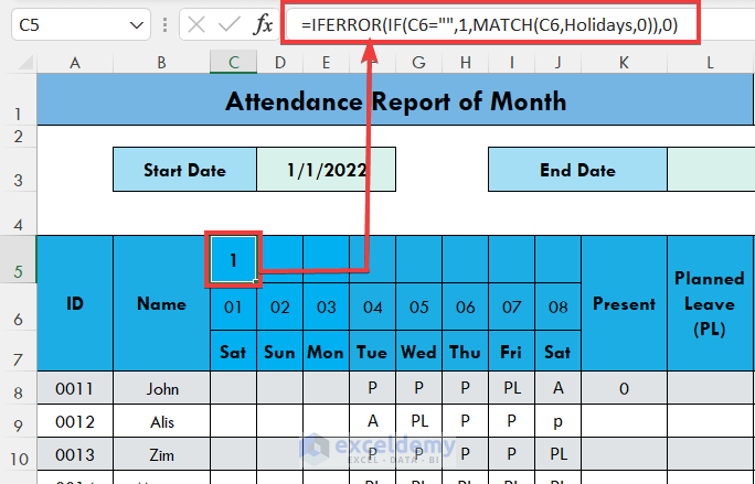
Put this formula into cell C5:

=IFERROR(IF(C6="",1,MATCH(C6,Holidays,0)),0)

Formula Explanation

MATCH(C6,Holidays,0) : The MATCH function will search the value of C6 in the Holiday list.
IF(C6=””,1,MATCH(C6,Holidays,0) : IF Function denotes that if the value of cell C6 is blank then insert 1 else search that in the Holiday list.
IFERROR(IF(C6=””,1,MATCH(C6,Holidays,0)),0) : It denotes that when the IF condition can’t give any values then it will give an error value and the IFERROR function works to give the value 0 instead of Error!.

Drag the formula to the remaining cells of the row.
The template will be like the screenshot below.

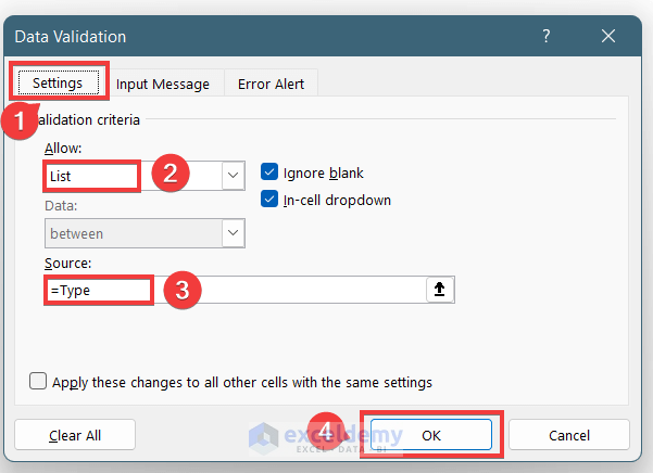
Step 7 – Setting up a Drop-down Menu for the Attendance Cells

Select all the attendance cells.
Go to the Data tab and pick Data Validation.

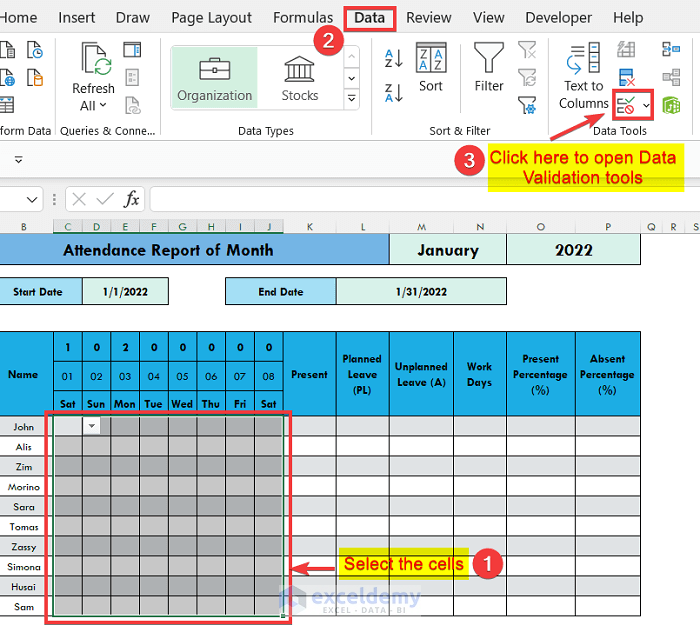
In the Data Validation window, remain in the Settings tab.
Select List from the Allow options.
Put =Type in the Source box.
Press OK.

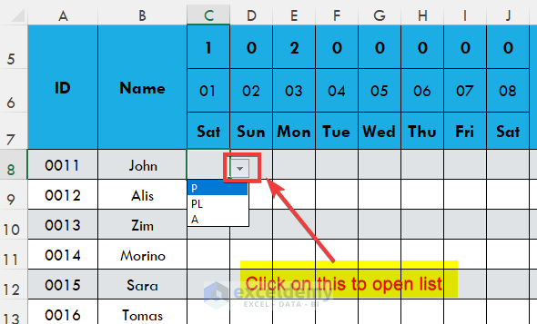
Go to any cells to insert attendance. You will find drop-downs next to the cell.
Select a value to insert. You can’t insert any other values.

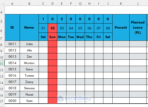
Step 8 – Highlighting Holiday Columns

Select all the cells of the attendance column.
Go to the Home tab, then to Conditional Formatting, and pick the New Rule option.

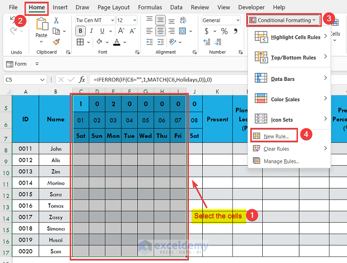
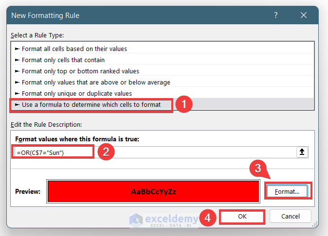
A window will appear named “New Formatting Rule”. Select the option “Use a formula to determine which cells to format” in the Rule Type.
Paste this formula into the Rule Description box:

=OR(C$7= "SUN")

Go to the Format option. Select a Red color as the Fill.
This will make the cells of the column red in which the 7th-row value is “Sun”. It will make Sunday columns red.

You will see the Sunday columns are in red.

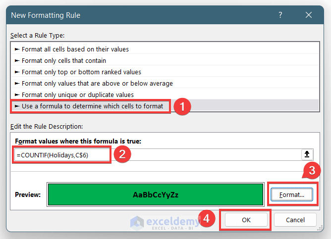
NOTES:: You can add any more days as weekends to mark as Red. Follow the same way to add again.

Insert one more conditional formatting to identify the office holidays from the list. Use this formula into the box:

=COUNTIF(Holidays,C$6)

Go to the Format option and select a Green color to fill the box.
Press OK.
Press Apply in the Conditional Formatting window to apply the formats.

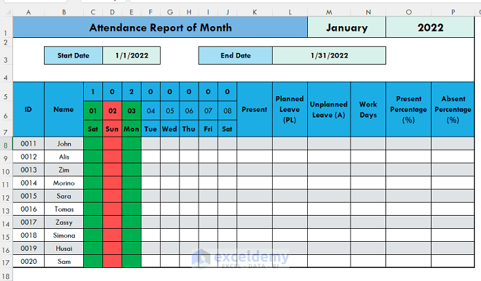
You will see the occasional holidays from the list are in green and Sundays are in red.

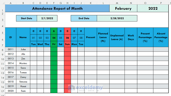
Select the month February to check whether the formatting is working.

Step 9 – Inserting Data in Attendance Cells

Insert data in the attendance cells to calculate the summary columns. You can write from the keyboard or use the drop-downs.

Step 10 – Inserting Formulas to Calculate the Total Attendance

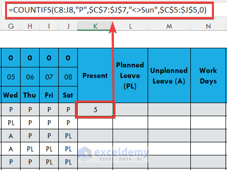
To calculate the total presence of the month or the week, insert this formula into the cell K8:

=COUNTIFS(C8:J8, "P",$C$7:$J$7,"<>Sun",$C$5:$J$5,0)

Formula Explanation

Using the COUNTIFS function, you will count the cells if they follow 3 conditions.
C8:J8, “P”: If the cell contains “P”
$C$7:$J$7,”<>Sun”: If the cell doesn’t contain “Sun”
$C$5:$J$5,0: If the cells are of value 0, it means it is not a holiday.

Copy the formula and paste it to the other cells of the column or use the Fill Handle icon to drag the formula.

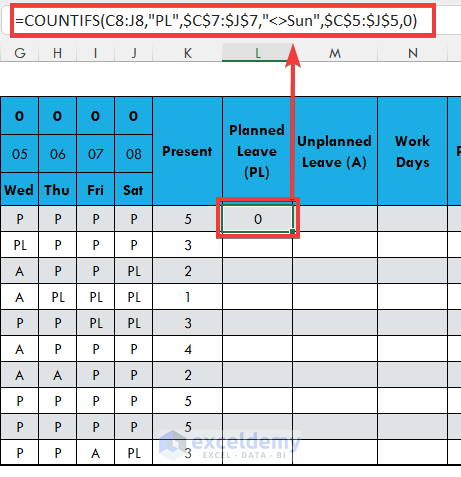
To calculate the total Planned Leave for the month or the week, insert this formula into the first cell:

=COUNTIFS(C8:J8, "PL",$C$7:$J$7,"<>Sun",$C$5:$J$5,0)

Copy the formula and paste it to the other cells of the column or use the Fill Handle icon to drag the formula.

To calculate the total Unplanned Absence (A) of the month or the week, insert this formula into the first cell:

=COUNTIFS(C8:J8, "A",$C$7:$J$7,"<>Sun",$C$5:$J$5,0)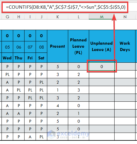

To calculate the total Work Days of the month or the week, insert this formula into the first cell:

=COUNTIFS($C$7:$J$7,"<>Sun",$C$5:$J$5,0)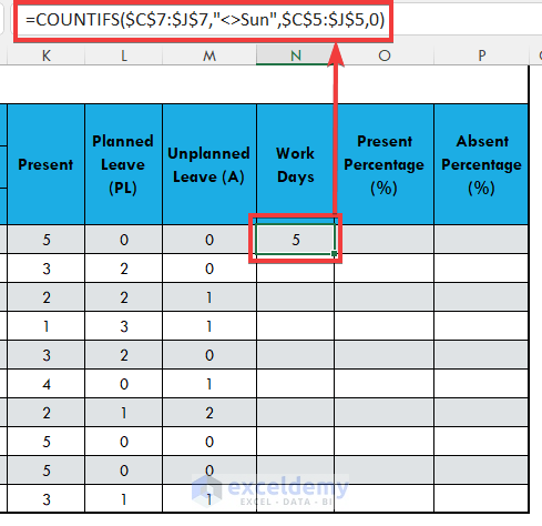

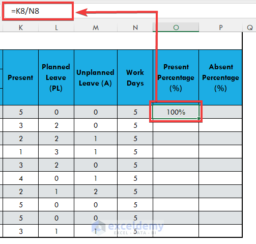
To calculate the Present Percentage, put the cells in the Percentage format.
Use this formula into the cell:

=K8/N8

This will divide the value of Total Presence by the Total Workdays.

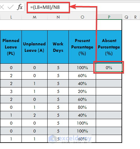
To calculate Absent Percentage, put the cells in the Percentage format.
Use this formula into the cell:

=(L8+M8)/N8

This will divide the value of Total Planned & Unplanned Absesnse by the value of Total Workdays.

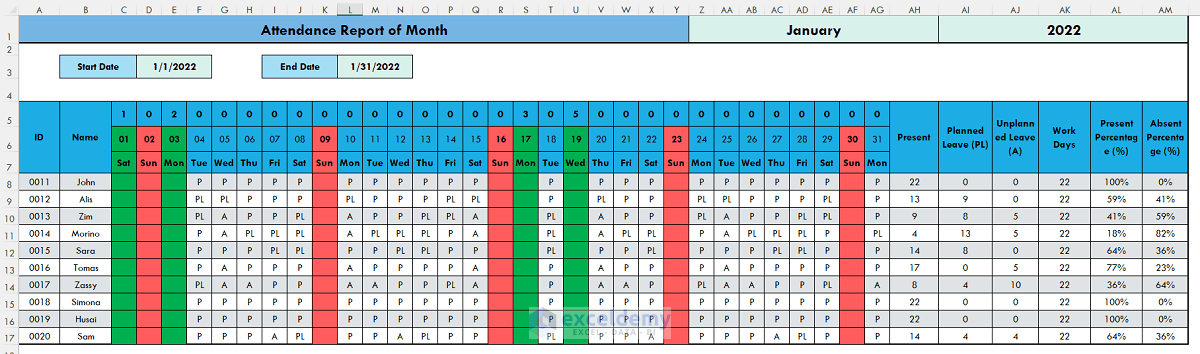
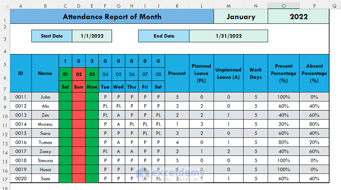
Your monthly attendance report is complete. You can track each employee’s attendance data easily.

Things to Remember

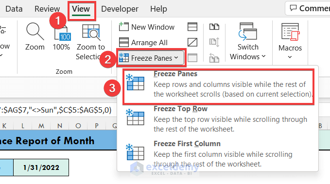
If the list is large, then you may face problems seeing the column header while scrolling. You can freeze the panes. in the Freeze Panes menu by selecting the Freeze Panes option here.

In the Holiday list, you can add or remove dates. After editing, do the Define Name step again.
This workbook will contain data for the full year. Simply copy the data of any month and use “paste value only” to another sheet to create a different worksheet for a different month. Then clean the attendance cells to track attendance for the next month.

Download the Free Template

You can download the Excel free template to Track Attendance from the following link.

Monthly Attendance Tracker.xlsx

<< Go Back to Formula List | Learn Excel

Get FREE Advanced Excel Exercises with Solutions!