How to Use TEXT Function in Excel (10 Examples)

In Microsoft Excel, the TEXT function is generally used to convert a numeric value to a specified format for various purposes. In this article, you’ll get to learn how you can use this TEXT function effectively in Excel with appropriate illustrations.

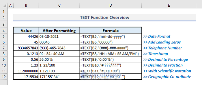
The above screenshot is an overview of the article, representing a few applications of the TEXT function in Excel. You’ll learn more about the methods and different formats to use the TEXT function with ease in the following sections of this article.

Introduction to the TEXT Function

• Function Objective:

TEXT function is used to convert a value to text in a specific number format.

• Syntax:

=TEXT(value, format_text)

• Arguments Explanation:

• Return Parameter:

A numeric value in a specified format.

How to Use TEXT Function in Excel: 10 Suitable Examples

1. Using TEXT Function to Modify Date Format

TEXT function is basically used to modify a date format in Excel. In the first argument, you have to input the date value or the cell reference of a date. Then you can define a proper date format by your own customization.

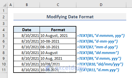
For example, in the following picture, a fixed date has been shown in different formats in column C. The first output, what we can obtain by typing the following formula:

You can copy the above formula and paste it into your spreadsheet to find the date format in a particular format if your cell B5 contains a date value or a date. You can display the dates in some other formats too by modifying the date codes like in the picture below.

2. TEXT Function to Connect Numerical Data to a Statement

In the picture below, an example of connecting a statement to numerical data in currency format is shown. The statement here is: ”You Have to Pay…“ and then the total sum of the food prices along with 4% VAT will be added after that statement. Technically we have to concatenate the two data by using an Ampersand (&) inside.

So in the output cell C9, the related formula with the TEXT function should be:

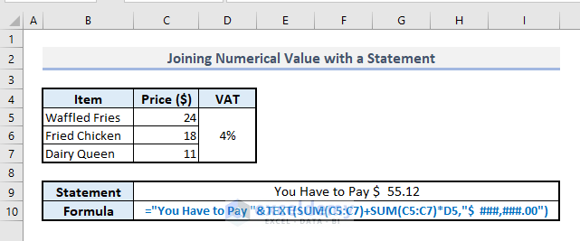
3. Joining a Date with a Statement by Combining TEXT and DATE Functions

Like the method shown in the previous section, we can also concatenate a text and a date by using Ampersand (&) as well as modifying the date format. The incomplete statement in the following screenshot is- “Today is…” and after this part, the current date has to be inputted in a proper format. So we can use the TODAY function here to include the current date and in the second argument of the TEXT function, we can modify the date code according to our wishes.

So, for our dataset, the related formula in the output cell B9 will be:

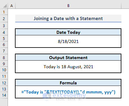
Read More: How to Use TEXT Function to Format Codes in Excel

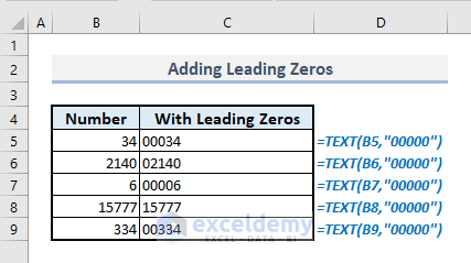
4. Adding Leading Zeros with TEXT Function in Excel

To keep or add leading zeros in a numerical value, the TEXT function can serve the purpose with the most suitable formula. In the following dataset, assuming that we want to resize all numbers to display a similar size by adding leading zeros before the numbers. All the numbers will be shown in five digits.

For the first instance, the required formula in Cell C5 will be:

After pressing Enter and auto-filling the rest of the cells in Column C with Fill Handle, you’ll get the desired results at once.

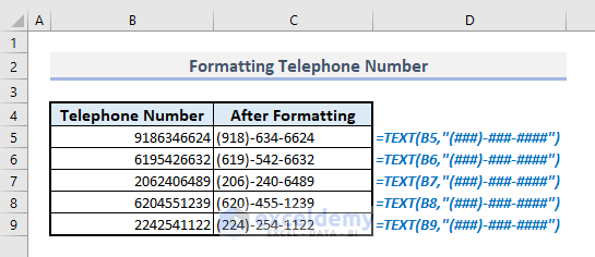
5. Formatting Telephone Number with TEXT Function

We can modify the telephone numbers in a particular format with the TEXT function. In the picture below, the relevant examples are being shown. While defining the format codes for telephone numbers, we have to replace the number characters with Hash (#) symbols.

So, the required formula for the first telephone number will be:

Press Enter and you’ll get the output with the defined format for a telephone number.

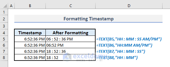
6. Use of TEXT Function to Format Timestamps

To format a timestamp, we have to use HH (Hour), MM (Minute), SS (Second), and AM/PM characters to define the required parameters. Here you have to keep in mind- in a 12-hour clock system, you have to input the AM/PM exactly in “AM/PM” text, not in “PM/AM” format at all, otherwise, the function will return with an unknown text value- “P1/A1” at the defined position in the timestamp.

In the following screenshot, a fixed timestamp has been shown in different but common formats after formatting. You can easily convert a 12-hour clock system to a 24-hour clock system and vice-versa by using this TEXT function.

Here, the first formula to format the timestamp in a 12-hour clock system is:

Now you can copy the formula and use it in your own Excel sheet with proper modifications for a timestamp.

Read More: How to Add Dashes to SSN in Excel

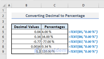
7. Converting Decimal to Percentage with TEXT Function

By using the TEXT function, you can convert a decimal number to a percentage more easily. You have to simply input “0.00 %” in the second argument. It’ll multiply the selected number or decimal defined in the first argument with 100 and add a percentage (%) symbol at the end.

The first output in the following table is the result of:

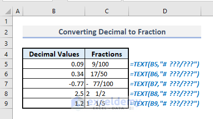
You can remove the decimals for the percentage by typing “0 %” only in the second argument. Or if you want to see the output with only one decimal place then you can use- “0.0 %” instead.

8. Converting Decimal to Fraction with TEXT Function

To convert a decimal value to a proper or a mixed fraction, you have to use the following formula for the decimal value in Cell B5:

In the second argument of the TEXT function, the format code is primarily assigned to return the output with the mixed fraction. But if the decimal value does not contain an integer value except 0 before the decimal point, then the function will return a proper fraction instead of a mixed fraction.

9. Converting Number to Scientific Notation with TEXT Function

Formatting a large string of digits in a number to a scientific notation is way too easy with the appropriate use of the TEXT function. You have to simply input an exponent with the letter ‘E’ after the defined characters for coefficients. By adding ‘+00’ after ‘E’, you have to denote the number of characters for the exponent power.

Based on the first output displayed in the picture below, the required formula with the TEXT function is:

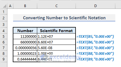
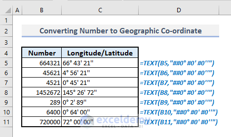
10. Converting Number to Geographic Coordinates with TEXT Function

To convert a number to a geographic coordinate, the related formula with the TEXT function in the output Cell C5 is:

Here you have to input the degree symbol in the second argument of the function by holding the ALT key and then pressing 0,1,7 & 6 one by one.

💡 Things to Keep in Mind

🔺 If you use hash (#) in the format_text argument, it’ll ignore all insignificant zeros.

🔺 If you use zero (0) in the format_text argument, it’ll show all insignificant zeros.

🔺 You must not forget to input quotation marks (“ “) around the specified format code.

🔺 Since the TEXT function converts a number to a text format, the output might be difficult to use later for calculations. So, it’s better to keep the original values in an additional column or row for further calculations if needed.

🔺 If you don’t want to use the TEXT function, you can also click on the Number command from the Number group of commands, and then you have to type the format codes by selecting the Custom format option.

🔺 TEXT function is really useful when you have to join a statement with a text in a specified format.

Download Practice Workbook

You can download the Excel workbook that we’ve used to prepare this article.

Concluding Words

I hope all of the suitable methods mentioned above to use the TEXT function will now provoke you to apply them in your Excel spreadsheets with more productivity. If you have any questions or feedback, please let me know in the comment section. Or you can check out our other articles related to Excel functions on this website.

<< Go Back to Excel Functions | Learn Excel