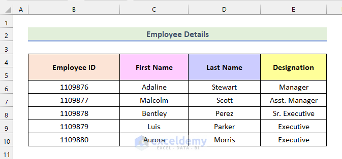
This is the sample dataset.
Step 1 – Creating a Support Sheet for an Automated Attendance Sheet in Excel
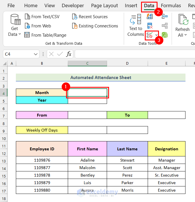
- In the Month Name column, enter the names of the 12 months.
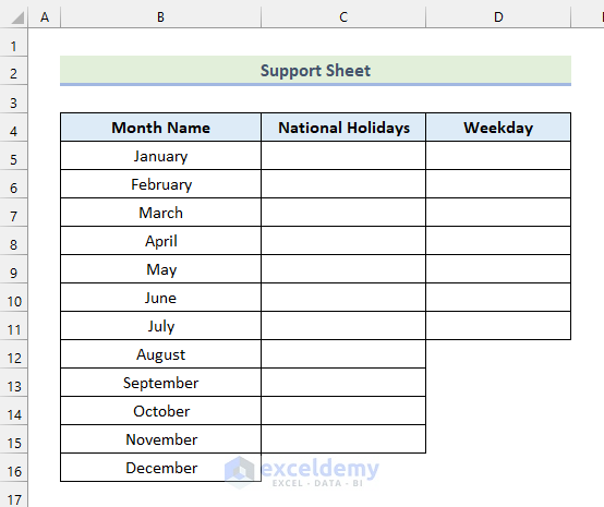
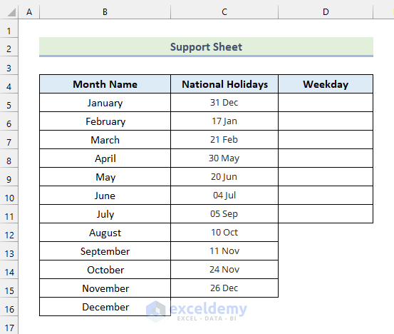
- In the National Holidays column, enter the list of National Holidays.
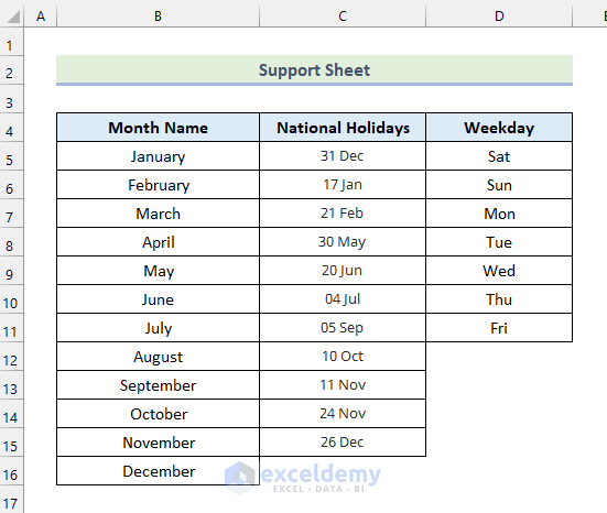
- Enter the name of the weekdays in the Weekday column.
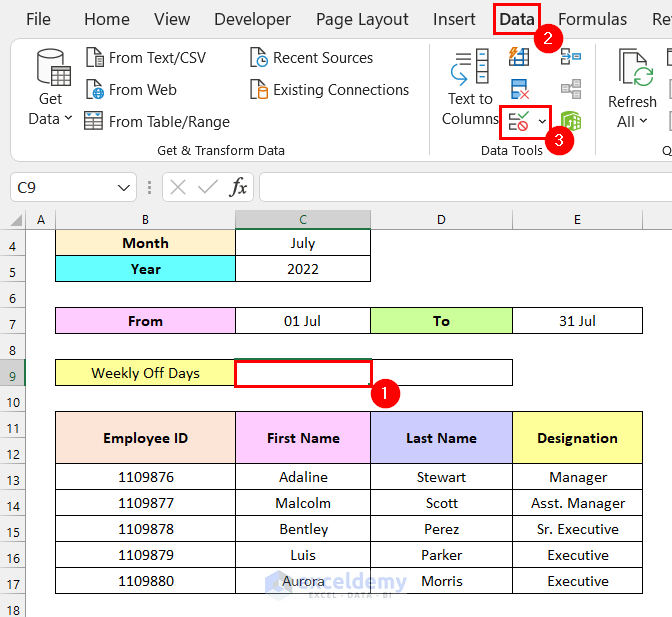
Step 2 – Creating a Month and Year List for an Attendance Sheet with Excel Data Validation
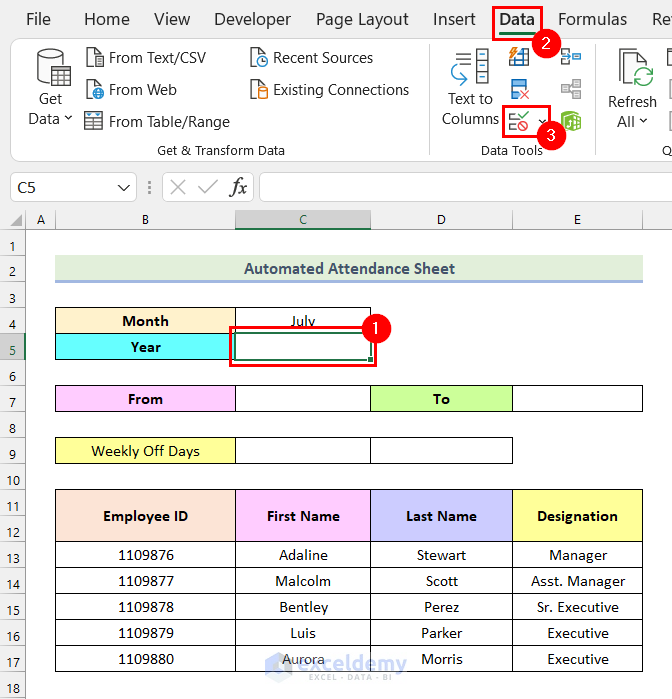
- Select C4.
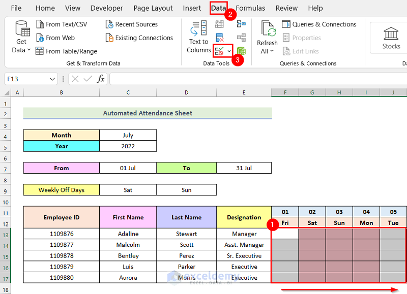
- Go to the Data tab.
- Click Data Validation in Data Tools.
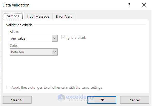
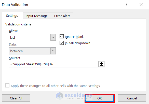
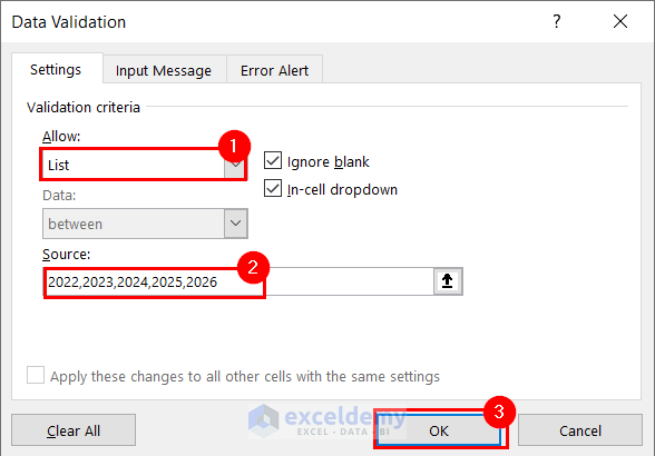
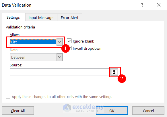
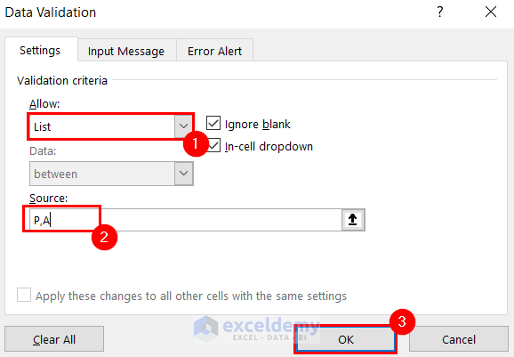
The Data Validation dialog box will open.
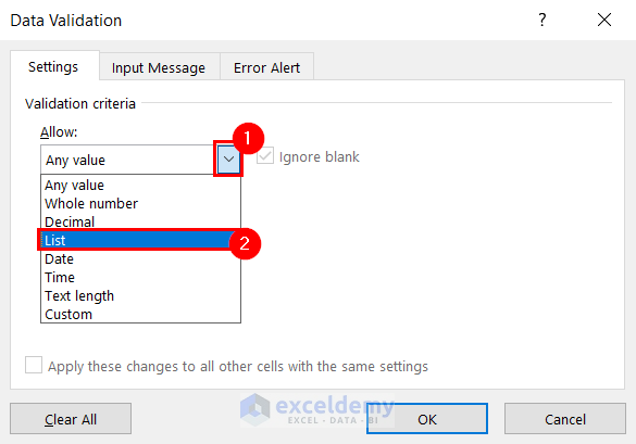
- In Allow, select List.
- In Source, click the upward arrow.
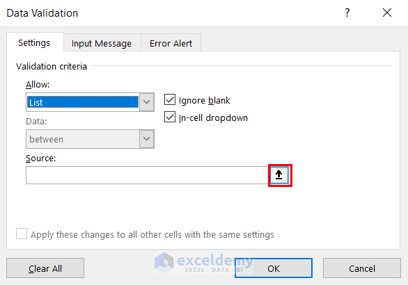
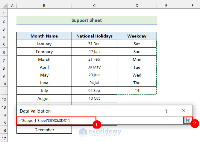
- Select all the months in the Month Name column of the Support Sheet.
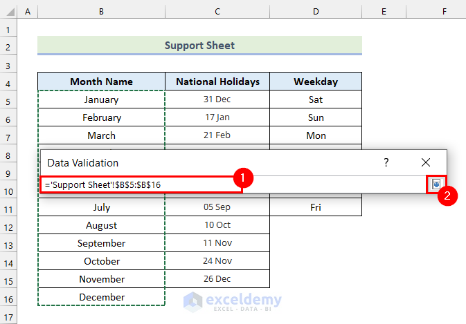
- Click OK.
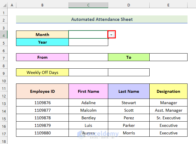
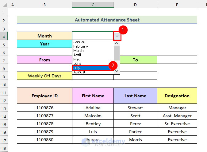
A drop-down icon will be displayed beside C4.
- Select a month. Here, July.
- Click C5.
- Go to the Data tab.
- Click Data Validation in Data Tools.
- Choose List.
- In the Source box, enter the years.
- Click OK.
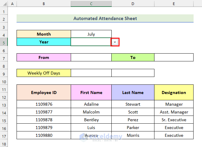
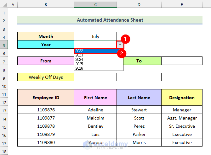
A drop-down button will be displayed beside C5.
- Choose a year. Here, 2022.
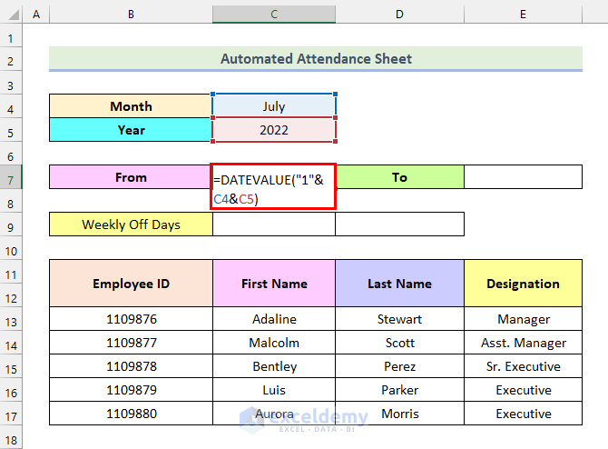
Create the start and end date of each month using the DATEVALUE function and the EOMONTH function.
- In C7 enter the following formula.
=DATEVALUE("1"&C4&C5)C4 indicates the chosen Month and C5 represents the selected Year.
- Press ENTER.
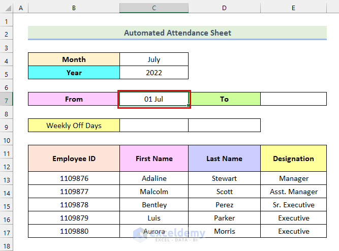
This is the output.
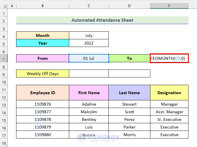
- In E7, enter the following formula.
=DATEVALUE("1"&C4&C5)C7 represents the start date of the month, and 0 means that the function will return the last date of the current month.
- Press ENTER.
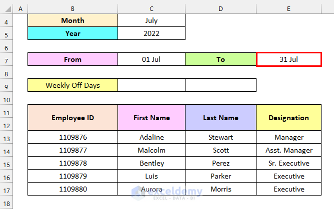
You will get the end date of the selected month. Here, 31 July (31 Jul).
Step 3 – Assigning Weekends in the Automated Attendance Sheet in Excel
- Select C9.
- Go to the Data tab.
- Select Data Validation.
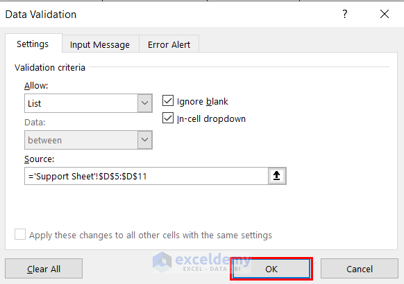
- In the Data Validation dialog box, choose List.
- In Source, click the upward arrow.
- Select the weekdays in the Weekday column of the Support Sheet.
- Click the downward arrow.
- Click OK.
- A drop-down button will be displayed beside C9. Click it.
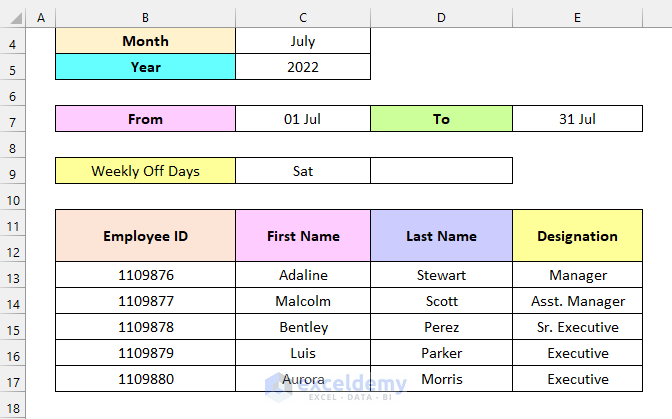
- Choose a weekly day off. Here, Saturday (Sat).
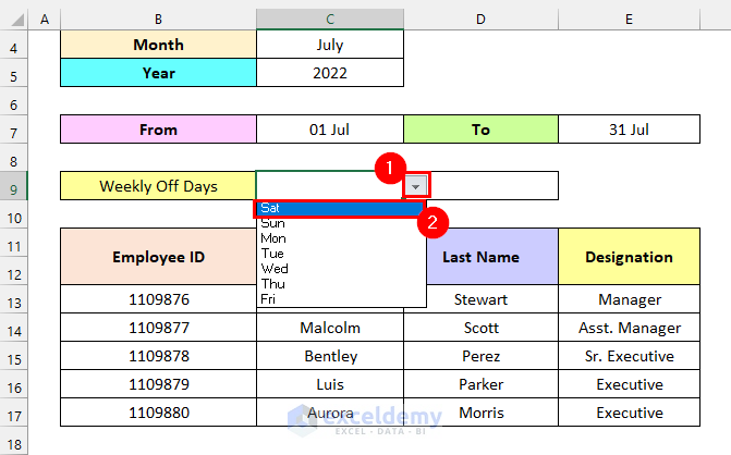
Saturday (Sat) is selected as the weekly day off.
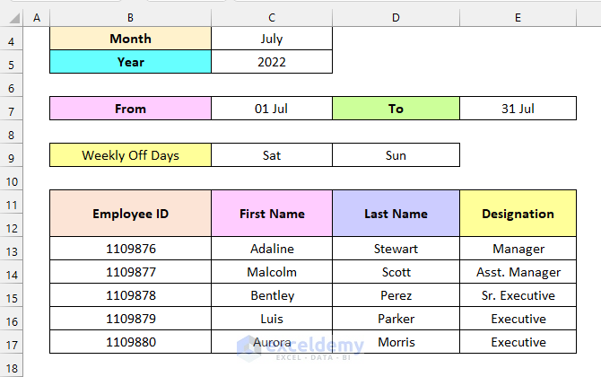
- Follow the same steps to select another weekly day off. Here, Sunday (Sun).
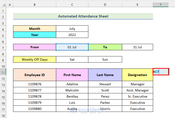
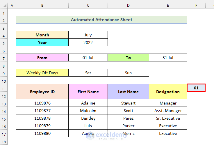
Step 4 – Entering Dates and Weekdays in the Attendance Sheet
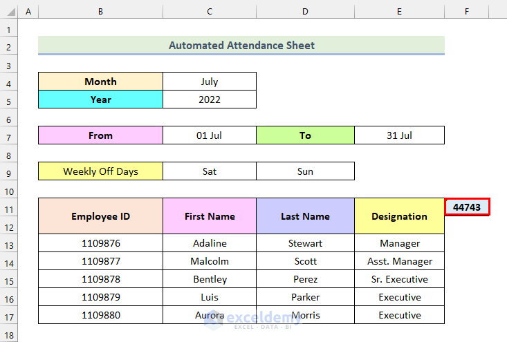
- In F11 enter the following formula.
=C7- Press ENTER.
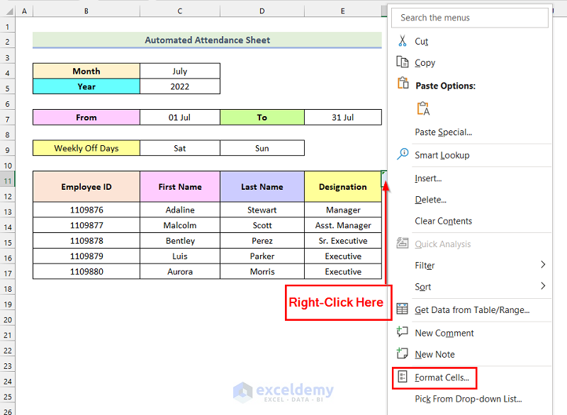
Change the cell format.
- Right-click F11.
- Select Format Cells.
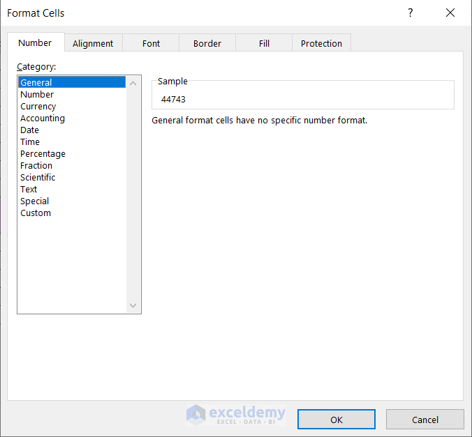
The Format Cells dialog box will open.
- Click Custom.
- Enter dd in Type.
- Click OK.
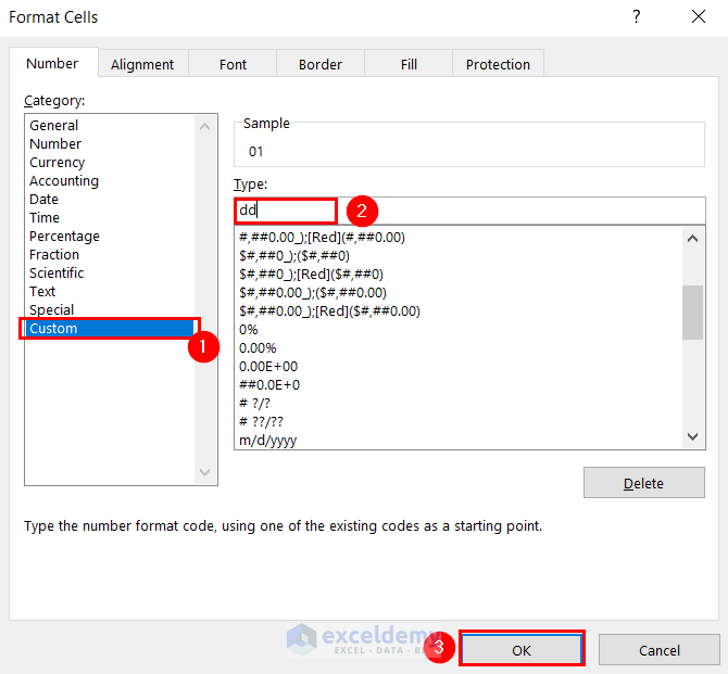
This is the output.
To obtain the rest of the days of the selected month, use the IF function. The logic is if the cell value is less than the end date of the month, the function increases the cell value by 1 (1 day). If this condition isn’t true, it replaces the cell with a blank.
- Use the following formula in G11.
=IF(F11<$E$7,F11+1,"")F11 is the 1st date of the month. $E$7 is the end date of the selected month.
Note: Absolute Cell Referencing for E7 ($E$7) was used.
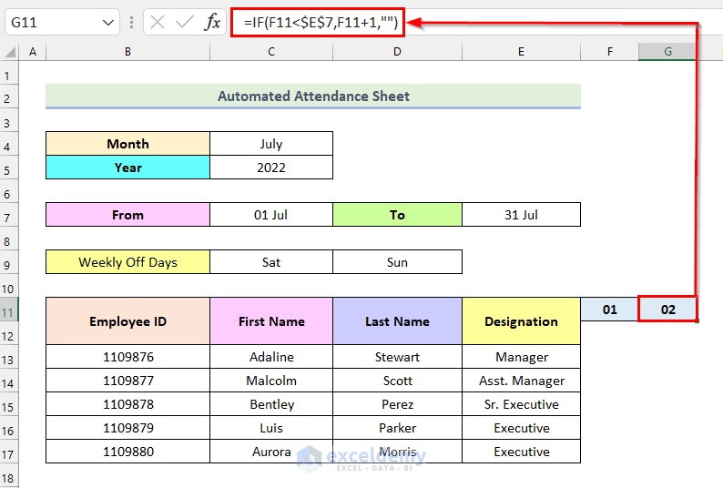
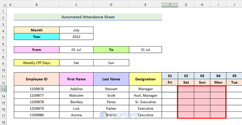
- Drag the Fill Handle to see the rest of the days of the selected month.

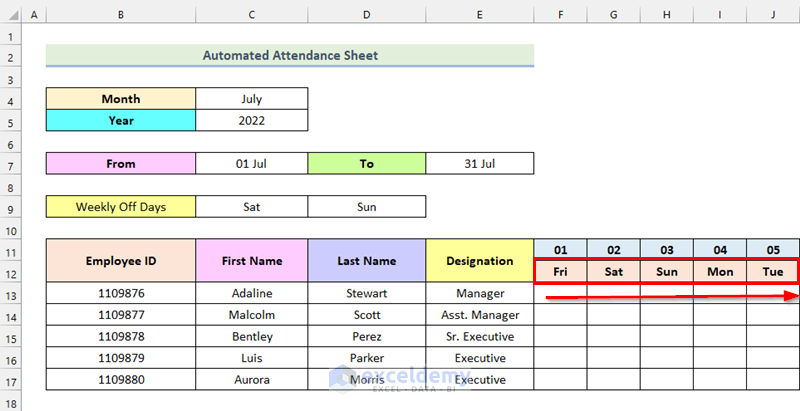
To enter the names of the weekdays:
- Enter the formula below in F12.
=TEXT(F11,"ddd")ddd is the date format. The output will contain the first 3 letters of weekdays.
- Press ENTER.
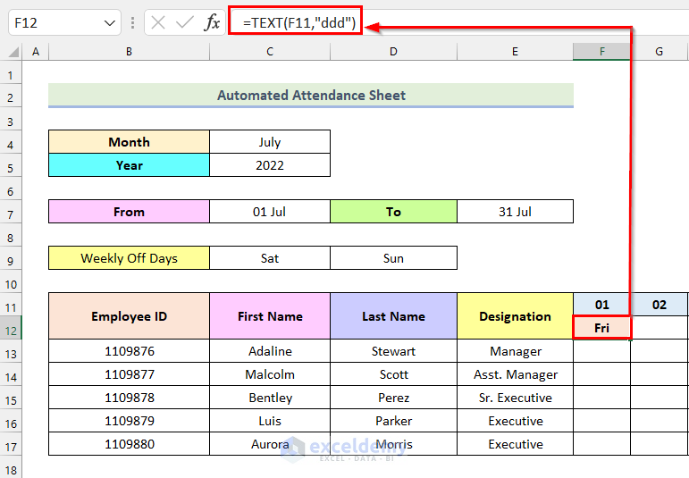
- Drag the Fill Handle to see the rest of the data.
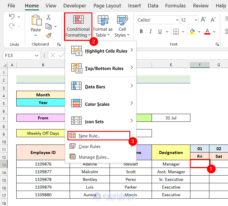
Step 5 – Using Conditional Formatting to Highlight Weekends
- Select F13.
- Select Conditional Formatting.
- Choose New Rule.
The New Formatting Rule dialog box will open.
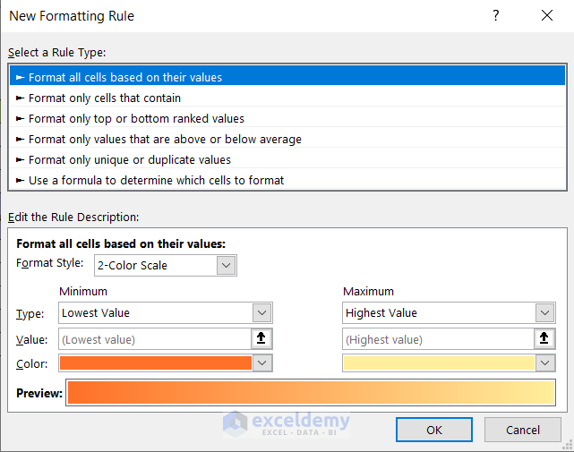
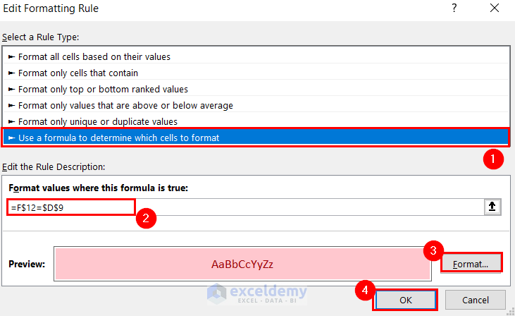
- Select Use a formula to determine which cells to format.
- Enter the following formula in Format values where this formula is true.
=F$12=$D$9$D$9 represents a Weekly Day Off (Sunday).
- Click Format option and select a formatting option.
- Click OK.
Note: Absolute Cell Referencing was used for D9 ($D$9). In F12 only the Row Number was fixed. This will allow you to copy the formatting to all cells in the same row.
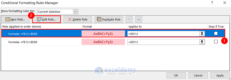
- Select the created rule.
- Click Duplicate Rule.
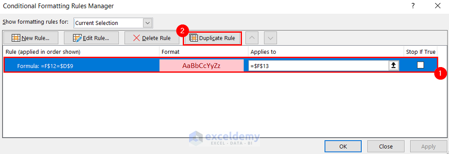
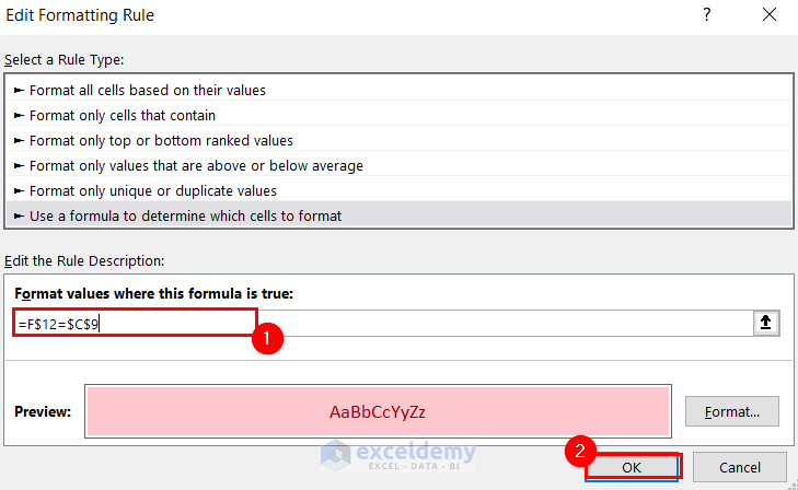
- Select the duplicated rule and click Edit Rule.
- Enter the following formula in Format values where this formula is true.
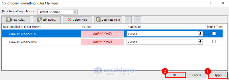
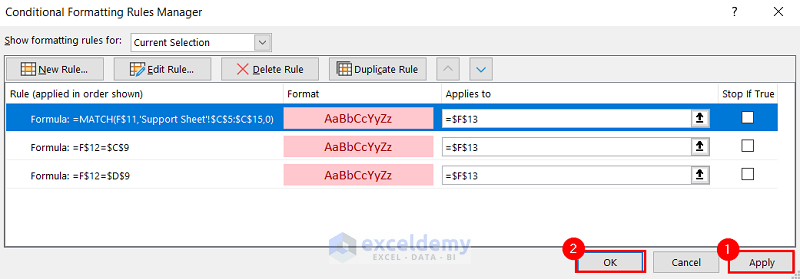
=F$12=$C$9$C$9 indicates the other Weekly Day Off (Saturday).
- Click OK.
- Click Apply in the Conditional Formatting Rules Manager dialog box.
- Click OK.
- Follow the previously described steps to open the New Formatting Rule dialog box.
- Select Use a formula to determine which cells to format.
- Enter the following formula in Format values where this formula is true.
=MATCH(F$11,'Support Sheet'!$C$5:$C$15,0)- Click Format option and select a formatting option.
- Click OK.
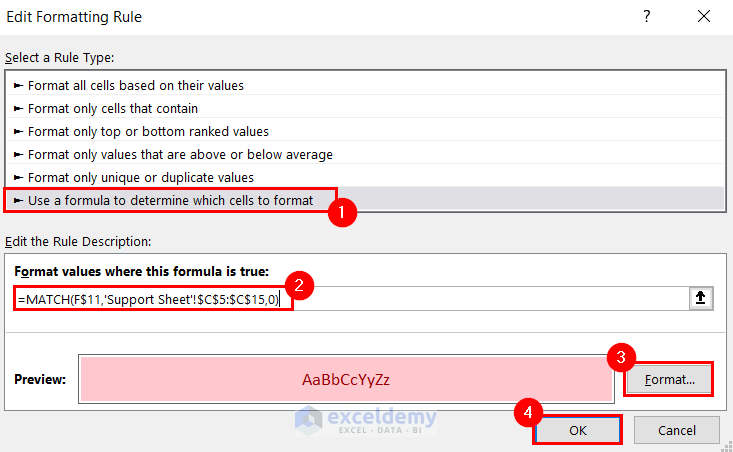
Note: The MATCH function was used to highlight National Holidays.
- Select Apply.
- Click OK.
- Select F13.
- Click the Format Painter icon.
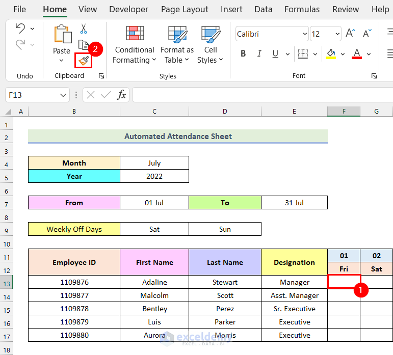
- Select F13:AJ17 to paste the copied formatting.
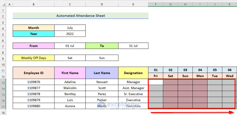
This is the output.
Step 6 – Entering Attendance Data in the Automated Attendance Sheet in Excel
- Select F13:AJ17.
- Go to the Data tab.
- Click Data Validation.
- In the Data Validation dialog box, choose List.
- In Source, enter P,A.
- Click OK.
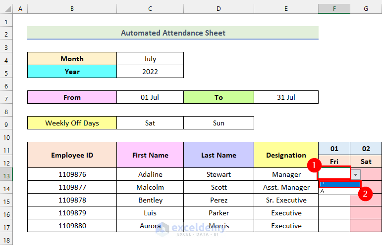
- Click the drop-down button beside F13.
- Choose P for present and A for absent.
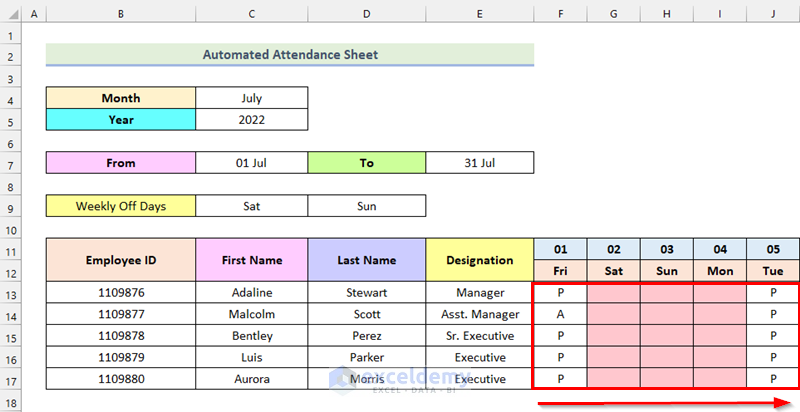
- Enter relevant attendance records in the other cells.
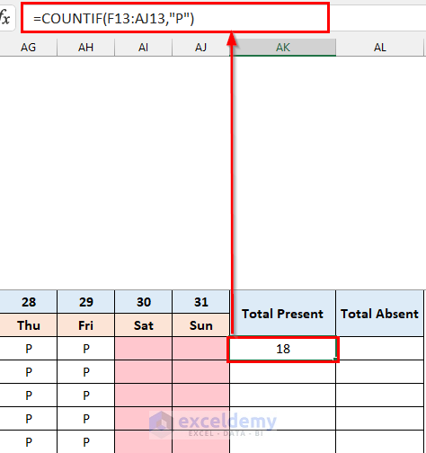
Step 7 – Using the Excel COUNTIF Function to Automatically Count Attendance
- Enter the following formula in AK13.
=COUNTIF(F13:AJ13,"P")F13:AJ13 is the range of the sum and P is the sum criteria.
- Press ENTER.
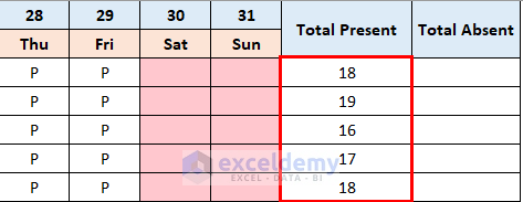
- Drag the Fill Handle to see the rest of the data.
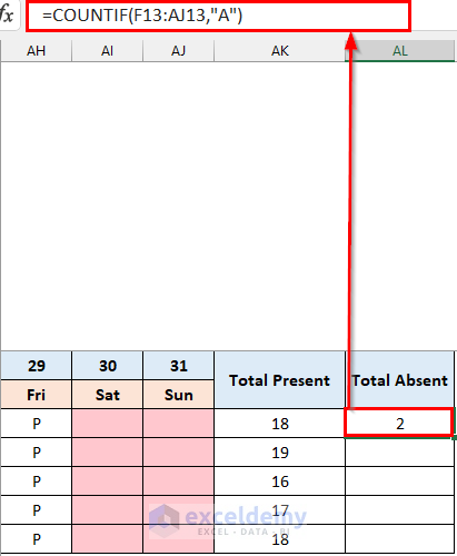
- Enter the following formula in AL13.
=COUNTIF(F13:AJ13,"A")A is the sum criteria.
- Press ENTER.
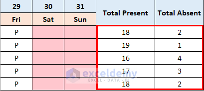
- Drag the Fill Handle to see the output.
Step 8 – Saving the Automated Attendance Sheet as a Template
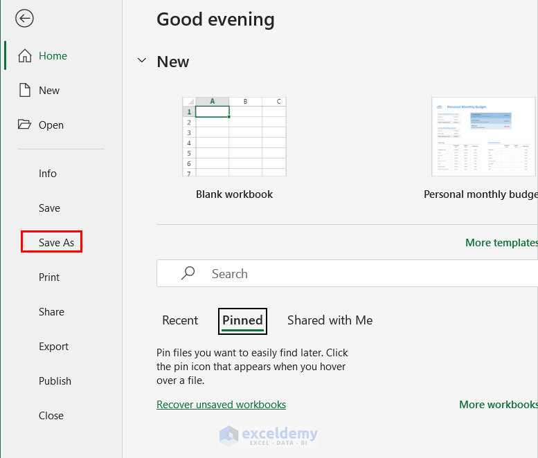
- Go to the File tab.
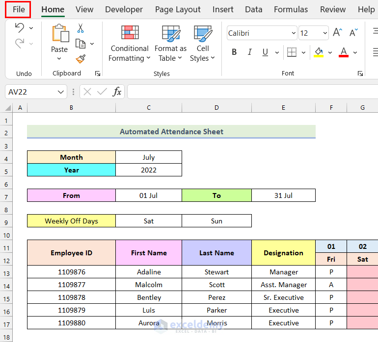
- Select Save As.
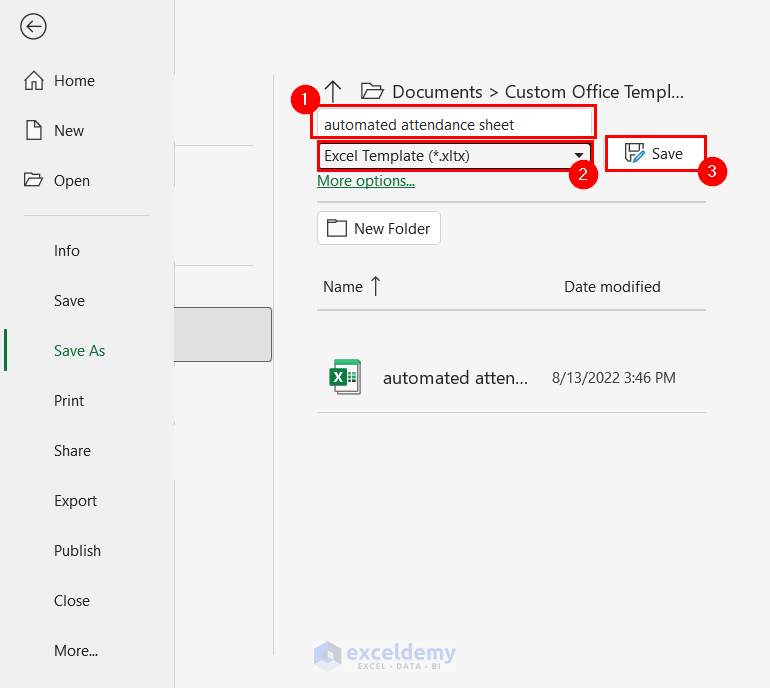
- Rename the file.
- Choose Excel Template (*.xltx).
- Click Save.
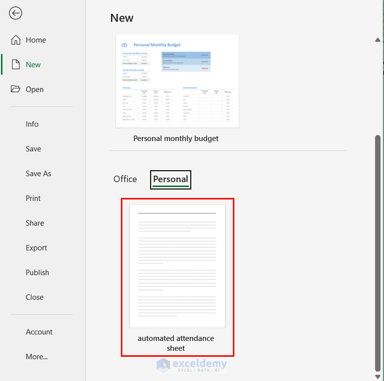
- To check the saved template, click New.
- Click the Personal tab.
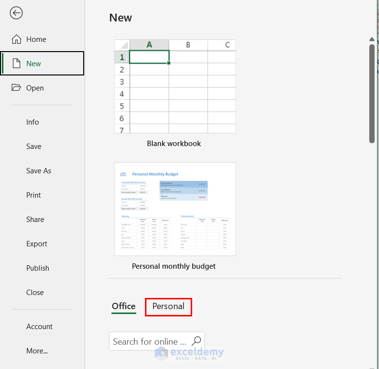
You can see your template.
Things to Remember
- While saving the file as a Template, use the default path suggested by Excel, which automatically saves the template to the Custom Office Template folder.
Download Practice Workbook
<< Go Back to Formula List | Learn Excel
Get FREE Advanced Excel Exercises with Solutions!

Hi, This really looks helpful. However, I need help on determining shift for each employee rather declaring same week off for all employees. For Eg. Employee A will work on Weekends (Sat,Sun) and avail week off on other two days in the week. Please help me on the same. Thanks.
Hi VIJAY,
Thank you for sharing your problem with us. As you wanted to determine each employee’s shift assuming that, their holiday can be any weekday, we have modified the attendance sheet. We hope this solution will meet your requirement.
1. First, you have to create a new table that will include the preferred work shifts of each employee.
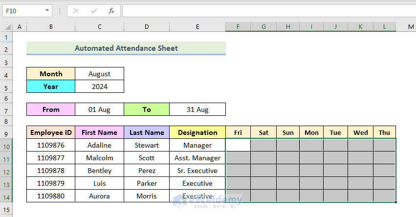

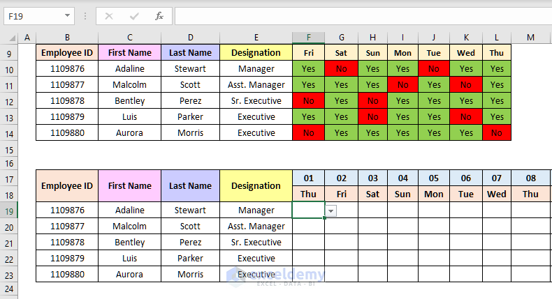
2. For simplicity, we are going to format these cells based on text value.
3. So, select the data range F10:L14.
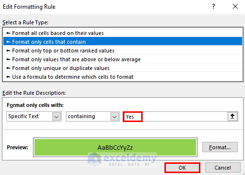
4. Now, from the Home tab go to Conditional Formatting and Select Format only cells that contain.
5. Then you have to set Yes as Specific Text.
6. Also, choose green as the format color.
7. Then, press the OK button.
8. Similarly, create another condition that if the cell contains the specific text No, the cell will be formatted as red.
9. Your selected cells should still be blank.
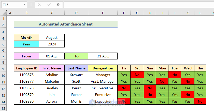
10. Now, to indicate the work shift, write Yes or No in these formatted cells.
11. And, you can see the cells are instantaneously formatted with green and red colors (You can also use Yes or No from the drop-down box instead of writing them manually).
11. Now, go to the attendance sheet and suppose, there is no condition in this Shift table.
12. Select the F19 cell and create a new condition.
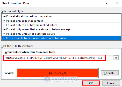
13. You have to select Use a formula to determine which cells to format as the New Formatting Rule.
14. Then, write the following formula in the formula box.
=INDEX($B$9:$L$14, MATCH($B19,$B$9:$B$14,0),MATCH(F$18,$B$9:$L$9,0))="No"15. Also, select a reddish format color and press OK.
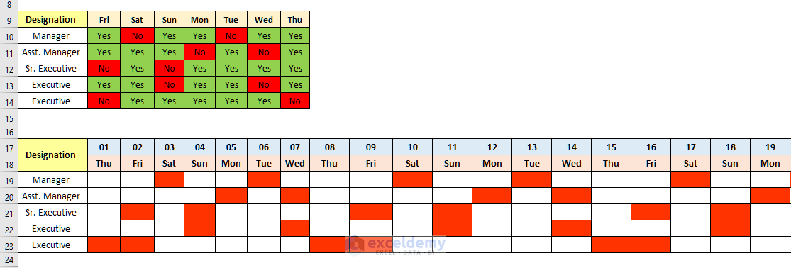
16. Then, use the Fill Handle to copy the conditional formatting for all cells as shown in the following image.
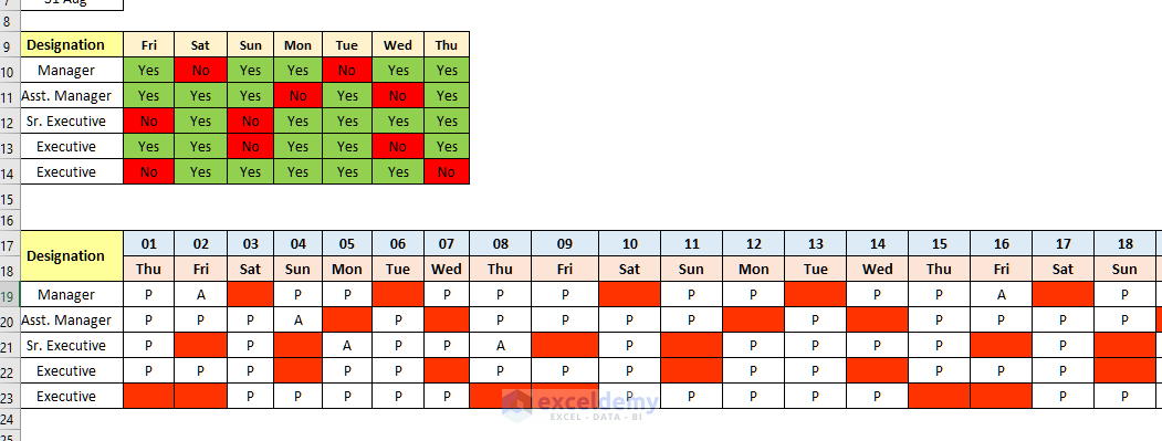
17. You can see, the Attendance table has been marked by each employee’s preferred off days.
18. Now, you can select Present (P) or Absent (A) for each employee.
You may need to modify the conditional format formula according to your data table. Be careful about relative and absolute referencing. You can also check the Excel file from the link below:
Answer.xlsx
We hope this comment has been useful to you. Have a nice day.
Regards
Sourav
Exceldemy.
This is super helpful but I’m having some issues with cell values copying over from month to month. I followed all the steps but when I enter a value for a particular day, it carries over to the same cell in all other months. For example, if I use the drop-down menu to set January 02 (cell I9) as ‘P’, when I switch to March it shows a ‘P’ in cell I9 as well. I’m not sure where I went wrong.
Hello Jessi,
It sounds like the issue is related to cell references being linked across months. This typically happens when the formula or cell is set to reference the same location across different months.
To fix it, check if absolute references (e.g., $I$9) are being used, and switch them to relative references (e.g., I9) for each month’s section. This way, each month will have independent entries.
Regards
ExcelDemy
Hello, thank you very much for this. May I know if we can change the data we add with a different month?
Hello Pasindu,
Yes, you can change the data to a different month. Just select the month from the dropdown list. Our months are listed in the Support Sheet.
Regards
ExcelDemy
Hello! If you select another month or year, isn’t it supposed to show empty cells? It still shows information from the previous month. How can I solve this problem, please?
Hello Brisa,
In the template, attendance entries are typed manually using a drop-down list. Changing the month or year does not clear those manual entries, Excel will keep whatever was previously entered until you delete them yourself.
If you want the cells to be empty when you change the month/year, you’d need to either:
1. Clear the old entries manually (Select the range → press Delete), or
2. Use VBA to automatically clear the attendance range whenever the month/year drop-down changes.
The current formula-free design in the article can’t reset old entries without VBA because the cells hold fixed values from your last input.
Regards
ExcelDemy