How to Use the SUMIFS Formula with Multiple Criteria in Excel – 11 Methods

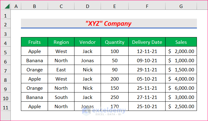
The sample dataset showcases Fruits, Region, Vendor, Quantity, Delivery Date and Sales.

You want to sum the values in Quantity or Sales based on different criteria.

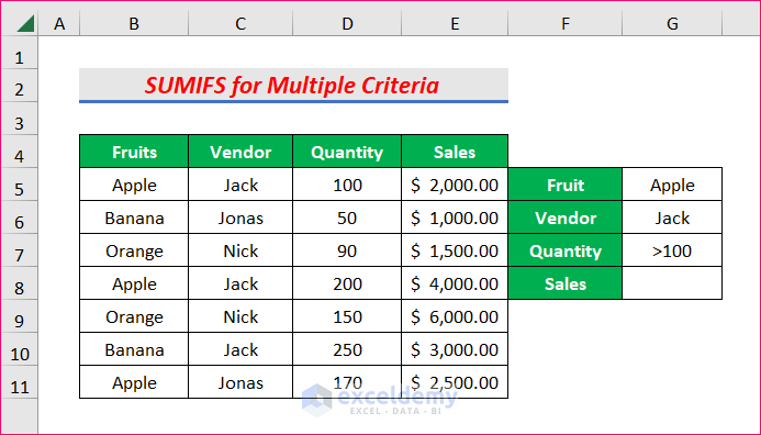
Method 1: Using the SUMIFS function for Multiple Criteria with a Comparison Operator

Use the SUMIFS function.

Step 1:
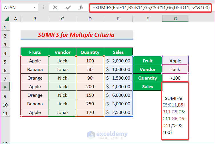
The output cell is G8
Enter the following formula in G8.

E5:E11 is the sum range
And B5:B11, C5:C11, and D5:D11 is the criteria range
G5, G6, and “>”&100 are the criteria.
If all criteria are met,  sales values will be summed.

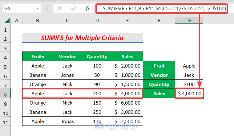
Press ENTER.

Result:
Then, you will get the total sales for Apple as Fruit, Vendor as Jack, and Quantity greater than 100.

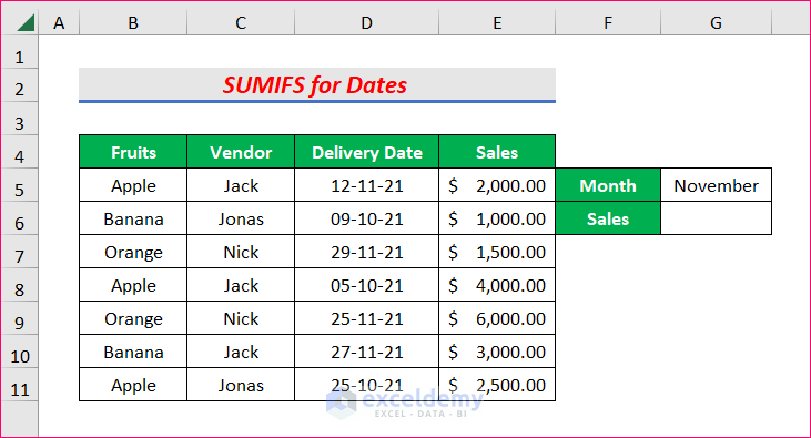
Method 2 – Using the SUMIFS Function for a Date Range

Use the SUMIFS function and the DATE function.

Step 1:
The output cell is G6.
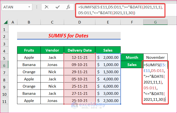
Enter the following formula in G6.

E5:E11 is the range of Sales, D5:D11 is the criteria range which includes the Dates.
">="&DATE(2021,11,1) is the first criteria: DATE will return the first date of a month.
"<="&DATE(2021,11,30) is used as the second criteria: DATE will return the last date of a month.

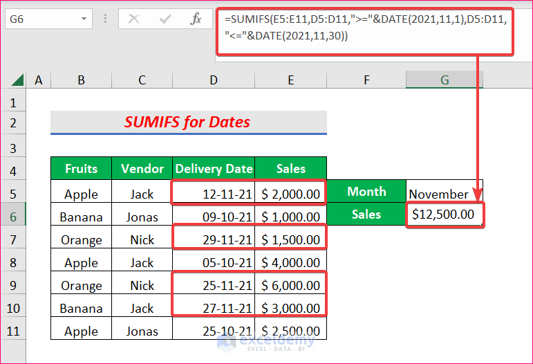
Press ENTER.

Result:
You will get the sum of sales for November.

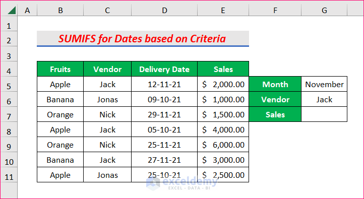
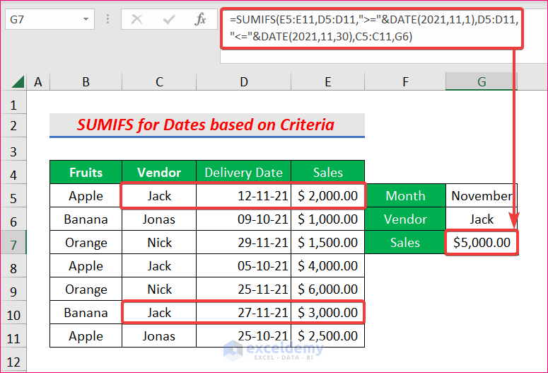
Method 3 – Using the SUMIFS Function for a Date Range based on Criteria

You want to sum Jack’s Sales in November.

Step 1:
Enter the following formula in G7.

E5:E11 is the range of Sales, D5:D11 is the criteria range which includes the Dates.
“>=”&DATE(2021,11,1) is the first criteria: DATE will return the first date of a month.
“<=”&DATE(2021,11,30) is used as the second criteria: DATE will return the last date of a month.
C5:C11 is the third criteria range and G6 is the criteria for this range.

Press ENTER.

Result:
This is the output.

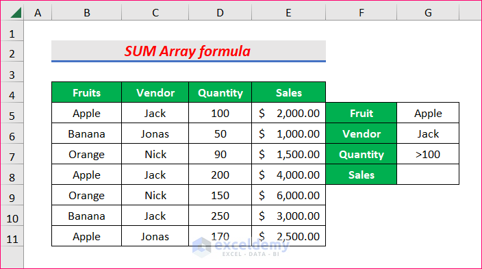
Method 4 – Using a SUM Array Formula for Multiple Criteria

Use the SUM function.

Step 1:
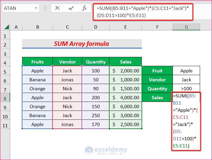
Enter the following formula in G8.

E5:E11 is the sum range
B5:B11=”Apple”, C5:C11=”Jack”, and D5:D11>100 are the three criteria based on which the sales will be added.

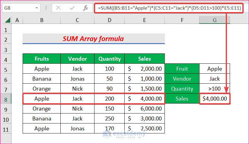
Press ENTER.

Result:
You will see the total sales for Apple as Fruit, Vendor as Jack, and Quantity greater than 100.

Note:
If you are using a version, other than Microsoft Excel 365, you must press CTRL+SHIFT+ENTER instead of ENTER.

Method 5 – Using the SUMIFS Function for Empty or Non-Empty Cells

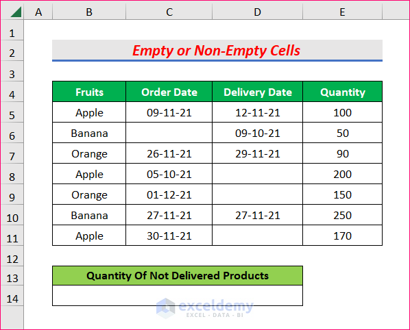
Step1:
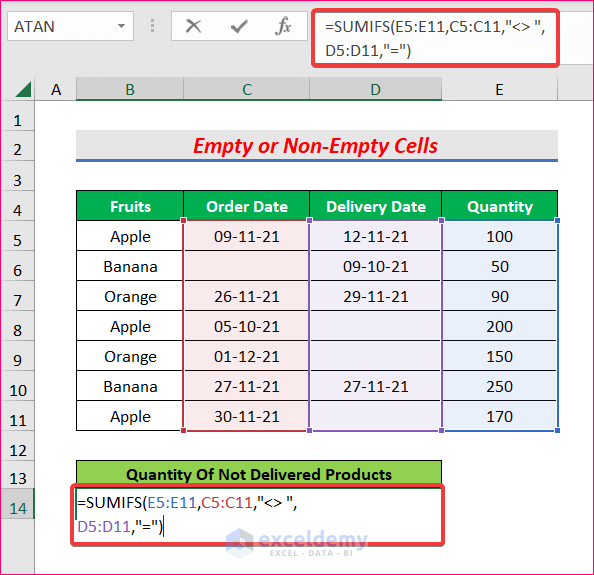
Enter the following formula in the output cell: B14.

E5:E11 is the sum range
C5:C11 is the range of Order Date and “<> “ is the criteria for this range which means not equal to Blank.
The range of Delivery Date is D5:D11 and “=” is the criteria for this range which means equal to Blank. ( You can use ” ” instead of “=” also)

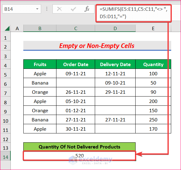
Press ENTER.

Result:
You will get the Quantity of Not Delivered Products.

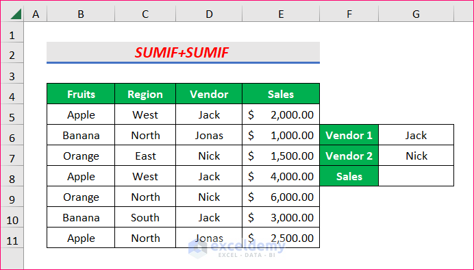
Method 6 – Using the SUMIF + SUMIF function for Multiple OR Criteria

Step 1:
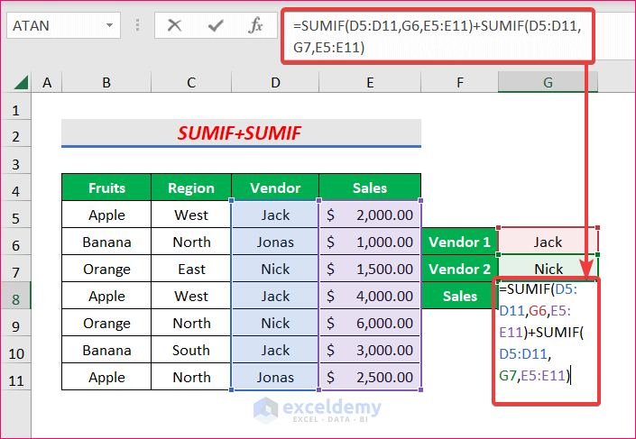
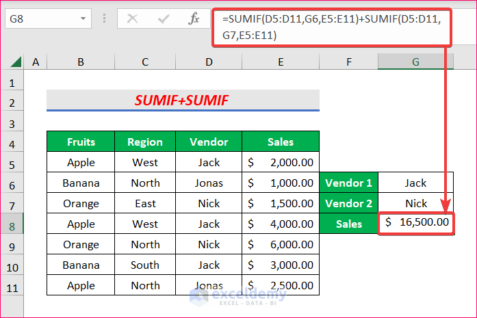
Enter the following formula in the output cell: G8.

This formula will add the Sales values for Vendors Jack and Nick and if one criterion is met, the values will be added.

Press ENTER.

Result:
You will see the Sum of Sales for Jack and Nick.

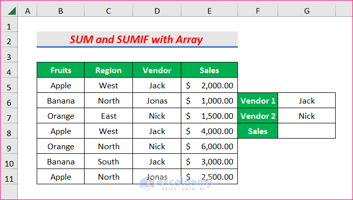
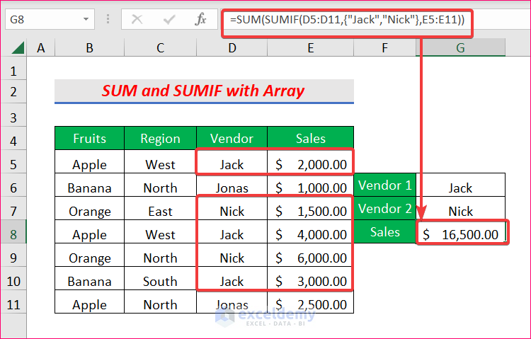
Method 7 – Using the SUM and SUMIF Functions with an Array Formula

Step 1:
The output cell is G8.
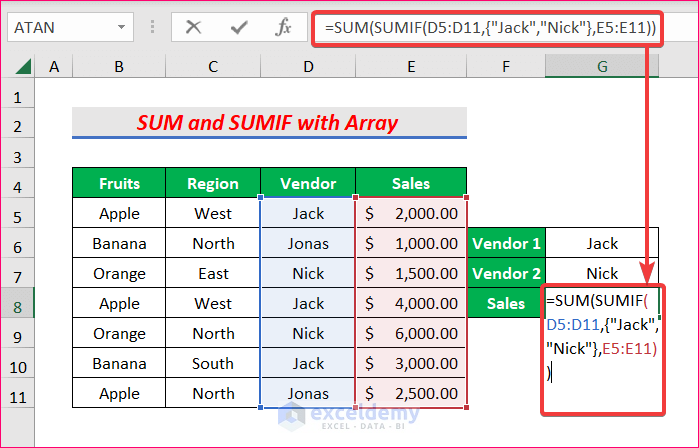
Enter the following formula in G8.

D5:D11 is the criteria range, {“Jack”, “Nick”} is the array of criteria and E5:E11 is the sum range.
Then SUM will add the Sales values for Vendors Jack and Nick and if one criterion is met, the values will be added.

Press ENTER.

Result:
You will see the Sum of Sales for Jack and Nick.

Note:
If you are using a version, other than Microsoft Excel 365, you must press CTRL+SHIFT+ENTER instead of ENTER.

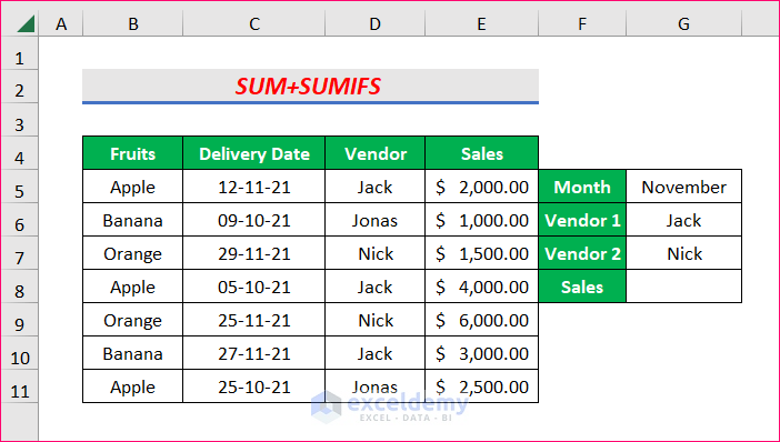
Method 8 – Using the SUMIFS + SUMIFS formula with Multiple Criteria

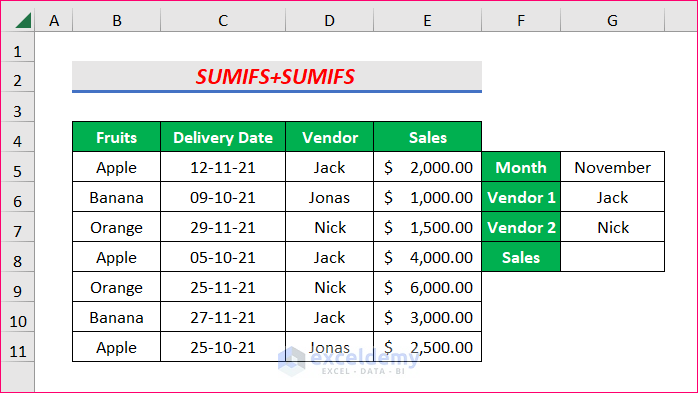
Step 1:
The output cell is G8
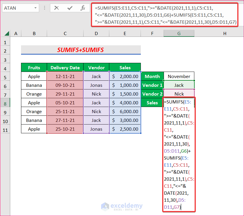
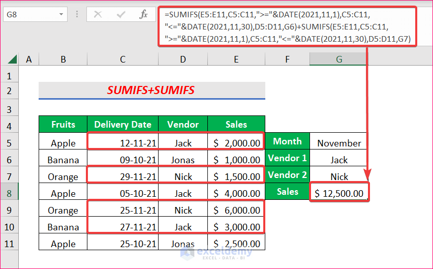
Enter the following formula in G8.

The two SUMIFS functions will add Sales value for Jack and Nick in November.

Press ENTER.

Result:
You will see the Sum of Sales for Jack and Nick in November.

Method 9 – Using the SUMPRODUCT and the SUMIF Function for Multiple Criteria

Use the SUMPRODUCT function and the SUMIF function.

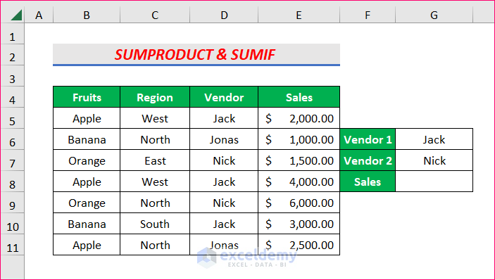
Step 1:
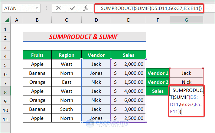
Enter the following formula in the output cell: G8.

D5:D11 is the criteria range, G6:G7 is multiple criteria in a range and E5:E11 is the sum range.

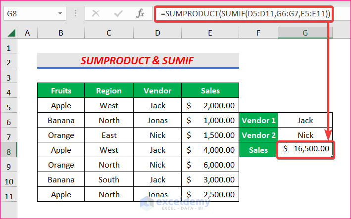
Press ENTER.

Result:
You will see the Sum of Sales for Jack and Nick.

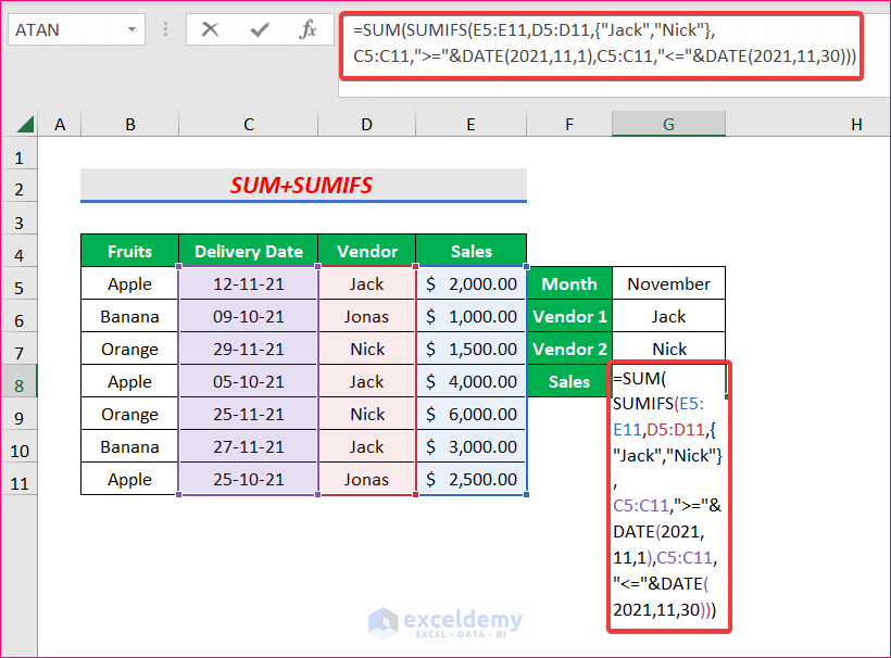
Method 10 – Using the SUM and the SUMIFS Function with an Array

Step 1:
Enter the following formula in the output cell: G8.

D5:D11 is the first criteria range, {“Jack”, “Nick”} is the array of criteria and E5:E11 is the sum range.

C5:C11 is the second and third criteria range
">="&DATE(2021,11,1) is the second criteria: DATE will return the first date of a month.
"<="&DATE(2021,11,30) is used as the third criteria : DATE will return the last date of a month.

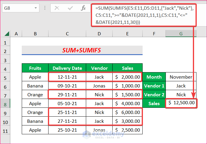
Press ENTER.

Result:
You will get the Sum of Sales for Jack and Nick in November.

Note:
If you are using a version, other than Microsoft Excel 365, you must press CTRL+SHIFT+ENTER instead of ENTER.

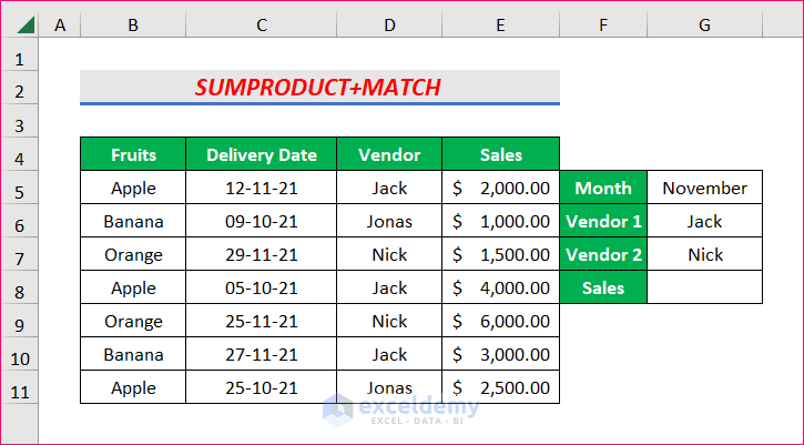
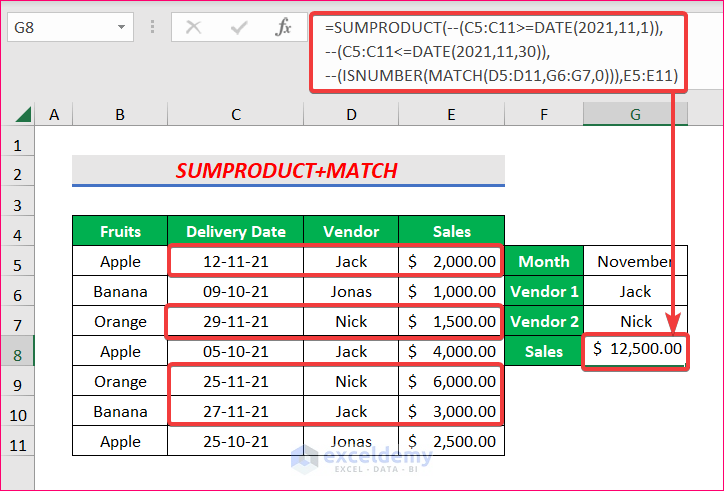
Method 11 – Using the SUMPRODUCT and the MATCH Functions for Multiple Criteria

Use the SUMPRODUCT function and the MATCH function.

Step 1:
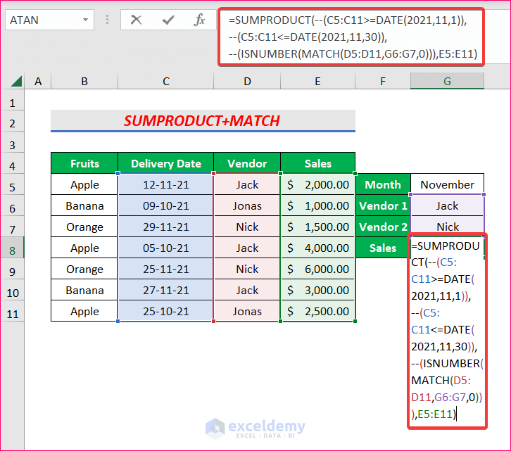
Enter the following formula in the output cell: G8.

Within the SUMPRODUCT function, there are three criteria, if they are fulfilled, it will return TRUE. Otherwise, FALSE. To convert the criteria into 1 or 0, a double negation(–) was used.

MATCH(D5:D11, G6:G7,0) matches Jack and Nick in the Vendor’s range.
ISNUMBER checks whether there is a number, and returns TRUE or FALSE.
After matching all the criteria, the SUMPRODUCT will add the values in E5:E11.

Press ENTER.

Result:
You will see the Sum of Sales for Jack and Nick in November.

Download Practice Workbook