How to Set Print Area for Multiple Pages in Excel (2 Ways)

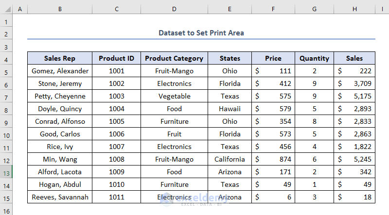
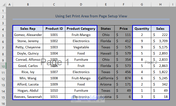
To demonstrate our methods, we’ll use the following dataset:

Method 1 – Using Set Print Area Option

STEPS:

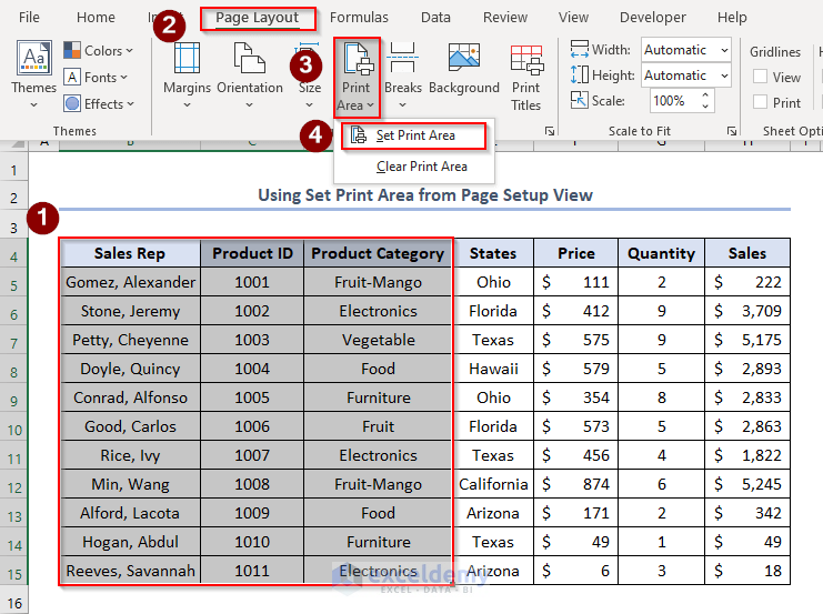
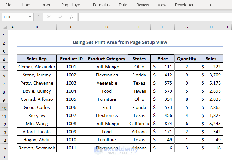
• Select the cells which we want to set as the print area for Page 1. Here, cells B4:D15.
• Click Page Layout > Print Area > Set Print Area.

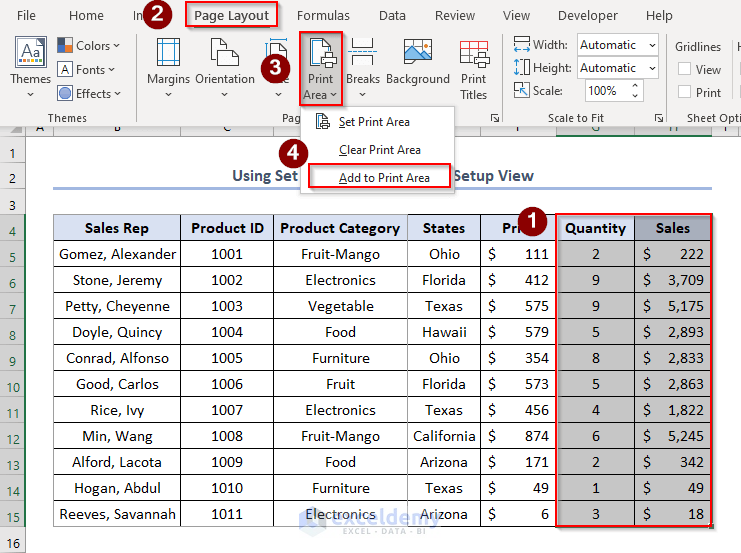
Let’s add some cells to the print area of Page 2.

• Select the cells to be added, here G5:H15.
• Click Page Layout > Print Area > Add to Print Area.

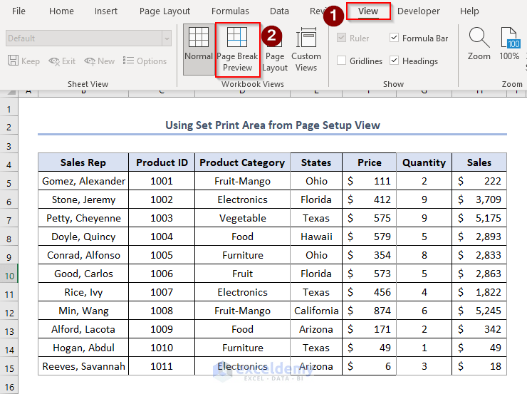
• To check the result, click View in the ribbon > Page Break Preview.

• In the Page Break Preview mode, the two print areas for Page 1 and Page 2 look like this:

• To revert to the original mode, select View > Normal.

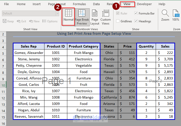
The normal view of the sheet returns.

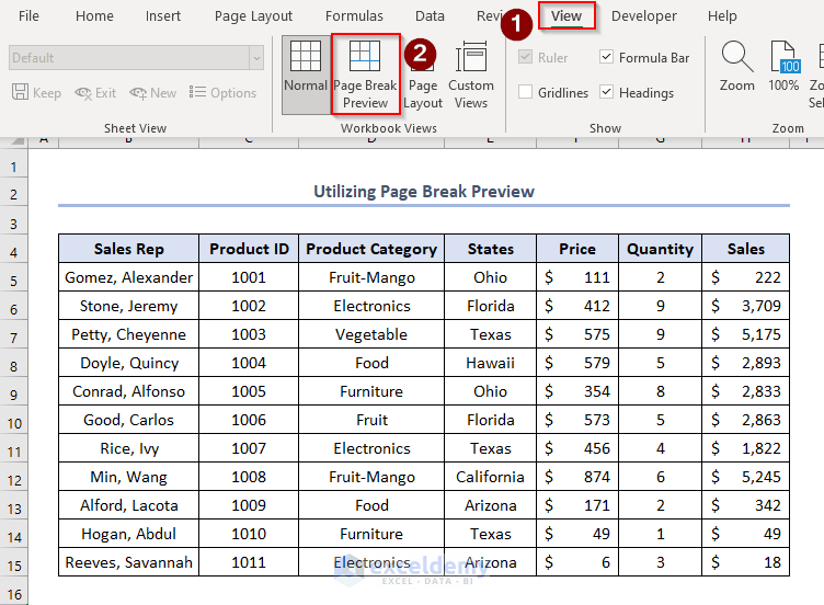
Method 2 – Applying Page Break Preview

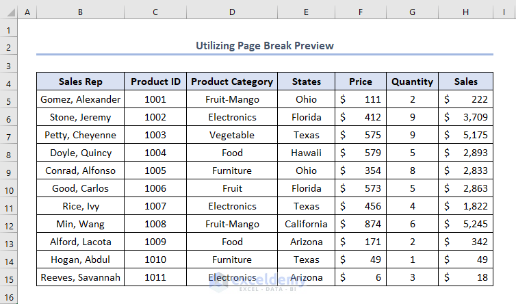
To demonstrate this method, we’ll use the following dataset:

STEPS:

• Click the View tab > Page Break Preview.

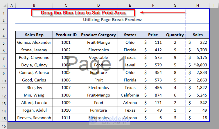
• The sheet including page breaks will display.
• Move the page break line toward the right or left to make customized pages. Suppose here we want to make Page 1 with column headers Sales Rep, Product ID, Product Category. Drag the page break line towards the left side until the Product Category column.

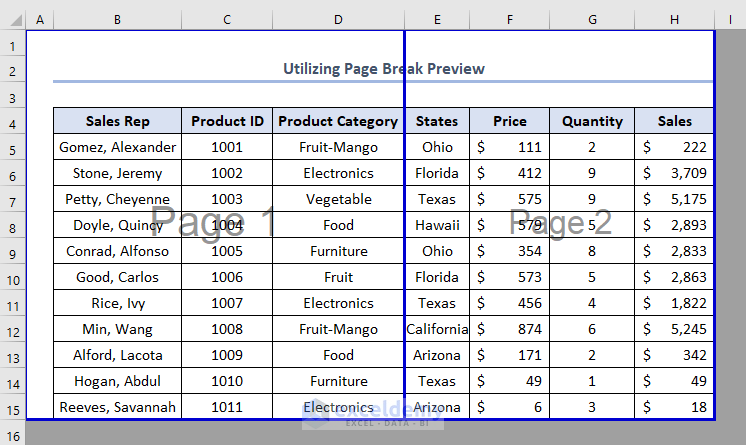
• After dragging the page break line, the two print areas for Page 1 and Page 2 are set.

Download Practice Workbook

Related Articles

• How to Print Selected Area in Excel
• How to Print Selected Area in Excel on One Page
• How to Set Print Area with Blue Line in Excel
• How to Center the Print Area in Excel

<< Go Back to Page Setup | Print in Excel | Learn Excel