How to Show Print Area in Excel: 4 Easy Methods

Method 1 – Using File Tab Option

Steps:

• Select the whole data table.
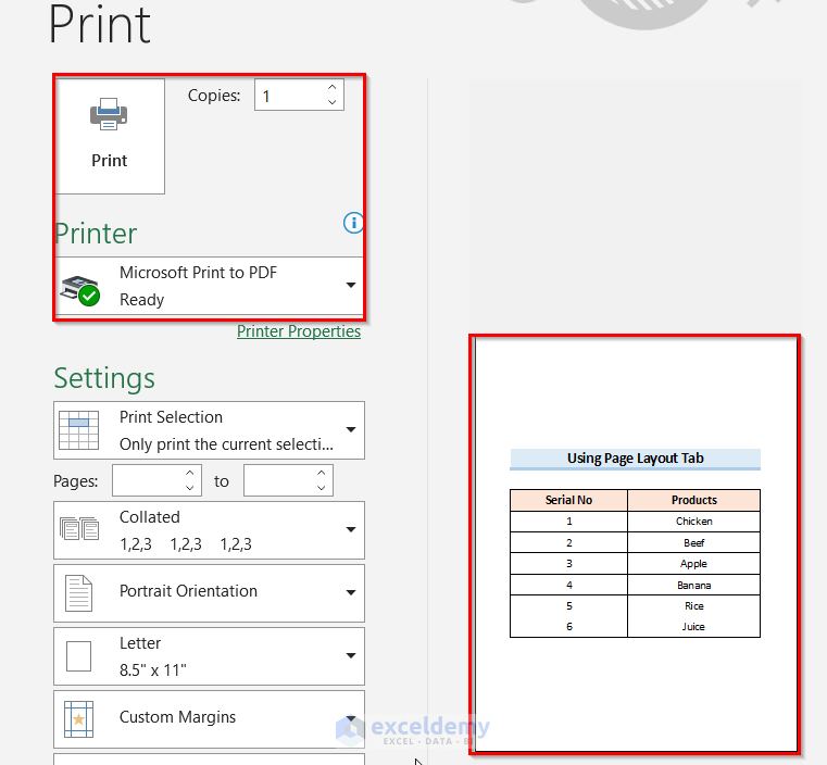
• Go to the File tab option.

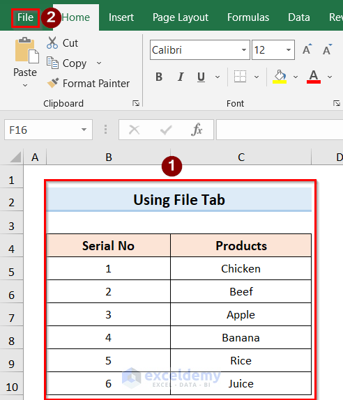
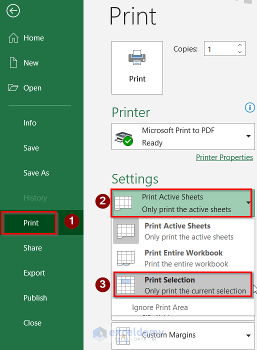
• Select the Print option.
• Go to the Print Active Sheets option and choose the Print Selection option.

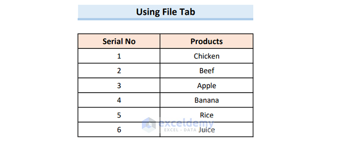
• You will get the below result.

Method 2 – Use of Page Layout Tab

Steps:

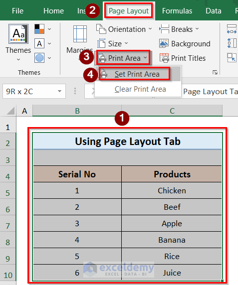
• Select the desired data table.
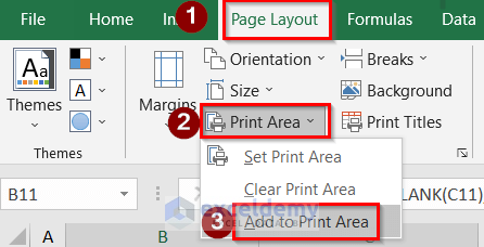
• Go to the Page Layout option.
• Choose the Set Print Area option from the Print Area option.

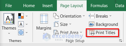
• Go to the Print Titles option on the side of the Print Area option.

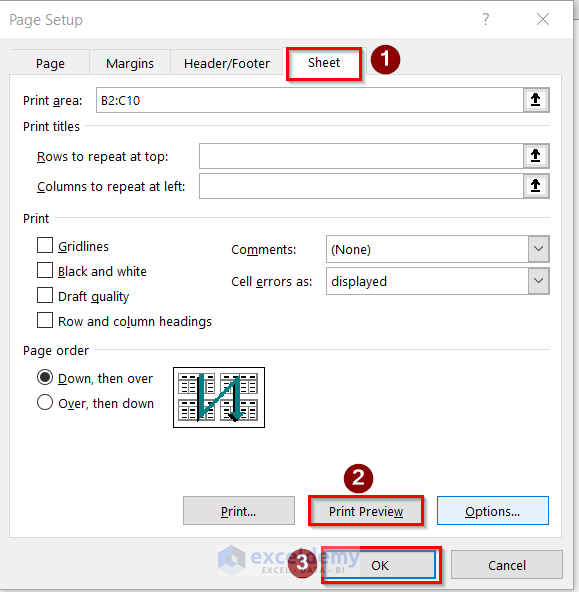
• The Page Setup dialog box will open on the window.
• Go to the Sheet, select the Print Preview option, and click OK.

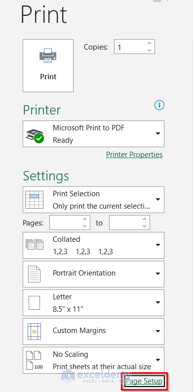
• If you want to open this Page Setup dialog box from the File tab then go to File > Print > Settings > Page Setup.

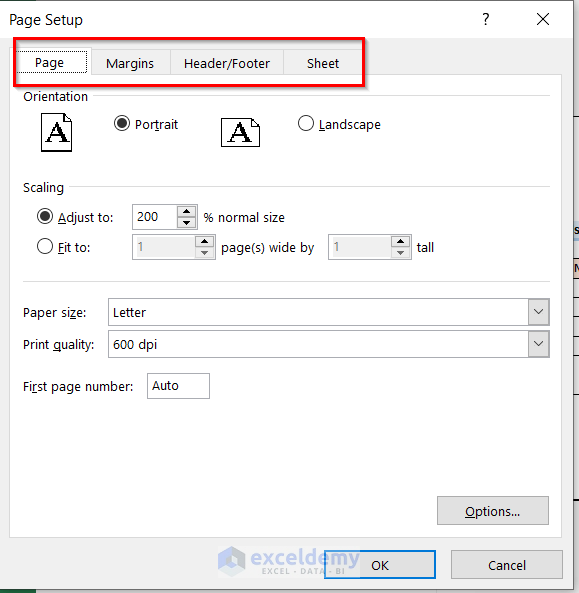
• You can customize the page setup, page margins, and header/footer of your printed area.

• Select the Print option.

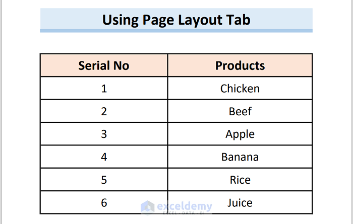
• You will get the result below.

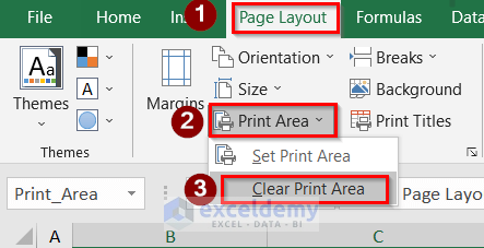
• If you want to clear the print area, go to the Page Layout option first.
• Select Clear Print Area from the Print Area option.

Method 3 – Adding Cells to Existing Printed Area

Steps:

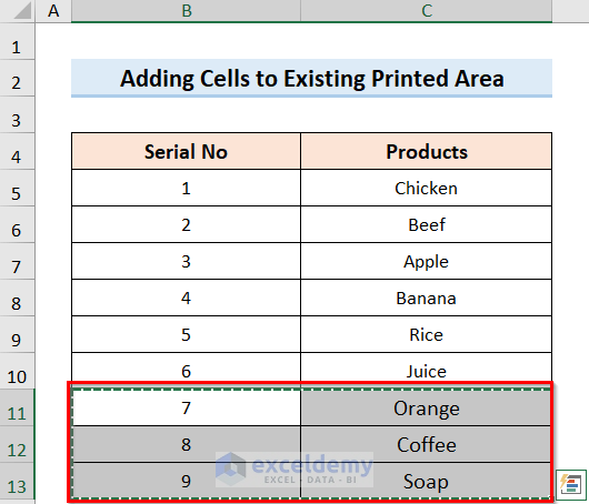
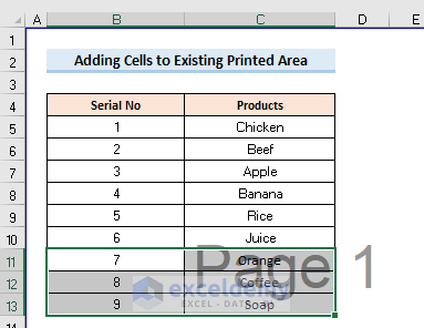
• Select the data you want to add in the printed area.

• Go to Page Layout>Print Area>Add to Print Area options.

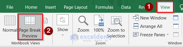
• Select the Page Break Preview feature from the View tab to show the data with desired page breaks.

• You will get the printed area similar to the below image.

Method 4 – Applying VBA Code

Steps:

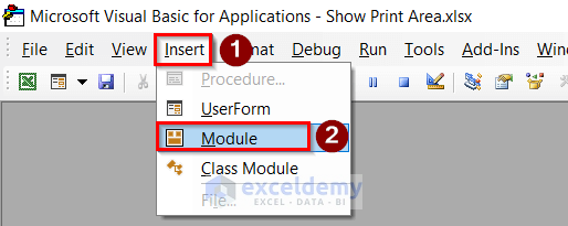
• Press Alt+F11 to open the VBA window.
• Select the Module option from the Insert tab.

• Insert the VBA code in the window.

Sub Print_Multiple_Range_in_One_Page()
Dim yRng1 As Range
Dim yRng2 As Range
Dim yNewWs As Worksheet
Dim yWs As Worksheet
Dim yIndex As Long
Application.ScreenUpdating = False
Application.DisplayAlerts = False
Set yWs = ActiveSheet
Set yNewWs = Worksheets.Add
yWs.Select
yIndex = 1
For Each yRng2 In Selection.Areas
yRng2.Copy
Set yRng1 = yNewWs.Cells(yIndex, 1)
yRng1.PasteSpecial xlPasteValues
yRng1.PasteSpecial xlPasteFormats
yIndex = yIndex + yRng2.Rows.Coun
Next
yNewWs.Columns.AutoFit
yNewWs.PrintOut
yNewWs.Delete
Application.DisplayAlerts = True
Application.ScreenUpdating = True
End Sub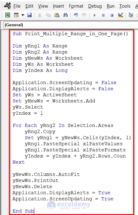

• Save the code and return the worksheet.
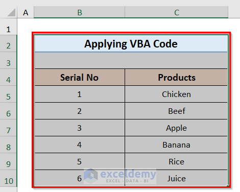
• Select the desired printed area.

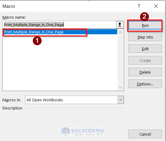
• The Macro tab will open on the screen.
• Run to apply the code to the desired selected area.

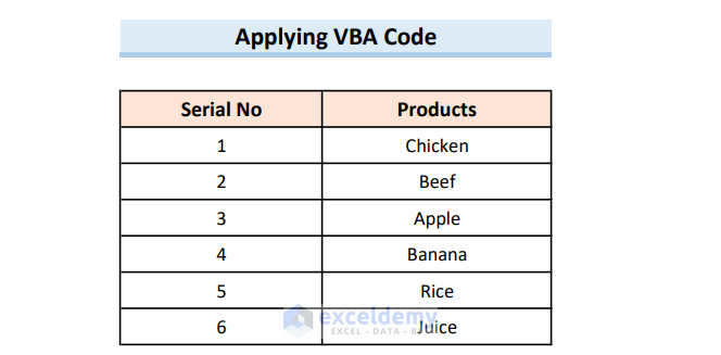
• You will get the result below.

Things to Remember

• The easiest method is the first method.
• In the case of method 3, remember that you have to print the area using the first two methods then if you want to add more cells or data to the printed area only then the Add to Print Area will appear on the screen.
• In the case of using VBA code, after inserting the code make sure to save it otherwise the code won’t work.

Download Practice Workbook

You can download the practice workbook from here.

Related Articles

• How to Change Print Area in Excel
• How to Delete Extra Pages in Excel
• [Solved:] Print Area Is Grayed Out in Excel
• [Fixed!] Excel Set Print Area Not Working

<< Go Back to Page Setup | Print in Excel | Learn Excel