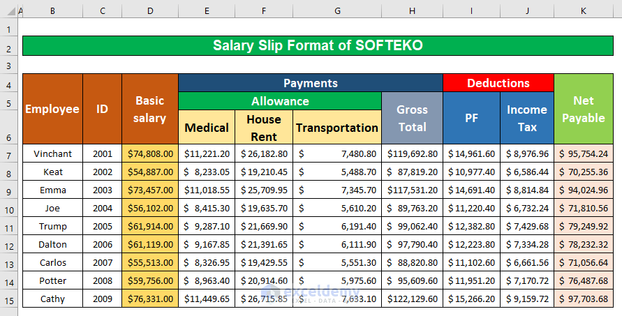
Let’s assume we have a large worksheet that contains the information about several Employee salary statements. The data for the Employee name, the Identification Number, the Basic Salary of the Employee, and the Medical, House Rent, and Transportation Allowances, Provident Fund, and Income Tax deduction are given in Columns B, C, D, E, F, G, I and J respectively. We will create a salary slip format in Excel.
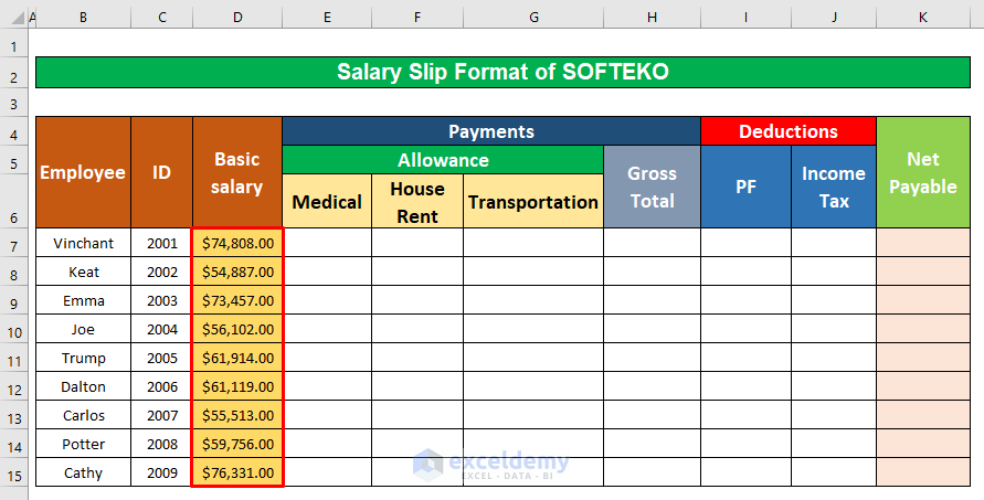
Step 1 – Create the Dataset for the Salary Slip Format
Insert the details of the employees, including the name of the Employee, the Identification Number, the Basic Salary of the Employee, and the Medical, House Rent, Transportation allowance, Provident Fund, Income Tax, etc.
Step 2 – Calculate Gross Totals Using Formulas in Excel
Let’s consider that the Medical allowance is 15%, the House rent allowance is 35%, and the Transportation allowance is 10% of the Basic salary of an employee.
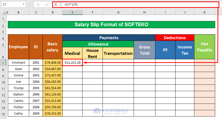
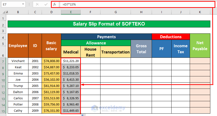
- Calculate the Medical allowance of the employees which is 15% of the Basic salary. Select cell E7 and insert the following formula into it:
=D7*15%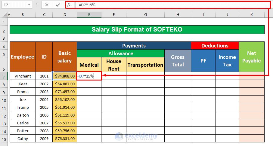
- Press Enter.
- AutoFill the formula to the rest of the cells in column E.
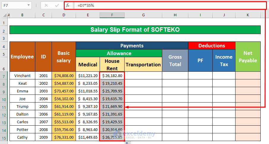
- Insert the following formula in cell F7 to get the Rent allowance:
=D7*35%- Press Enter on your keyboard.
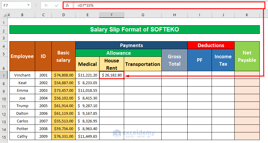
- AutoFill the formula to the rest of the cells in column F.
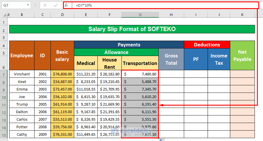
- Select cell G7 and insert the following formula for the transportation allowance:
=D7*10%- Hit Enter.
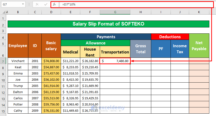
- AutoFill the formula to the rest of the cells in column G.
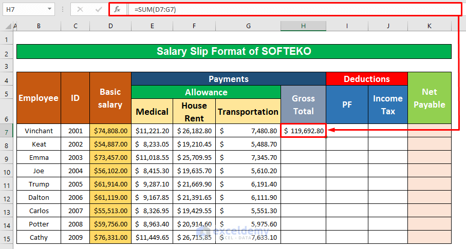
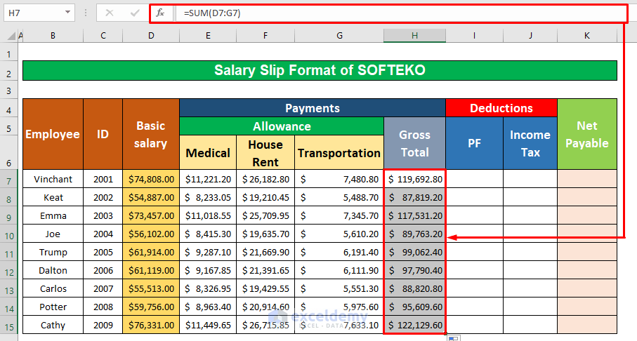
- Select cell H7 and copy the following function to get the gross total:
=SUM(D7:G7)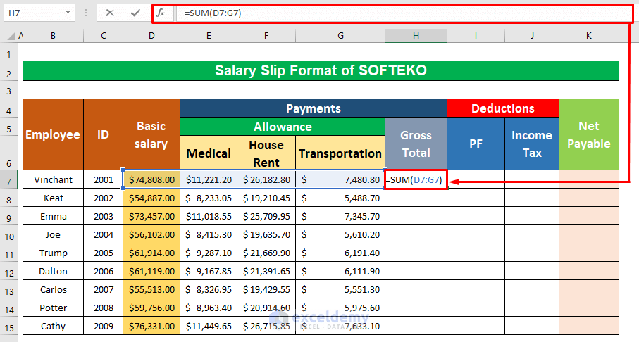
- Press Enter.
- AutoFill to the rest of the cells in column G.
Step 3 – Calculate Net Payable Values to Complete the Salary Slip Format
The Provident Fund and Income Tax will be deducted from the Gross Total salary and become the Net Payable salary. Let’s say the Provident Fund is 20% and the Income Tax deduction is 12% of the Basic salary of an employee.
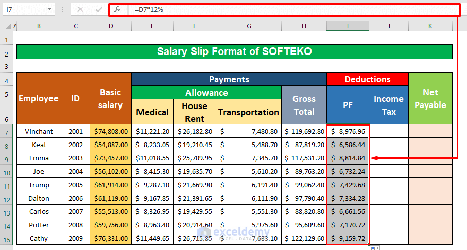
- Input the following formula in cell I7:
=D7*20%- Hit Enter.
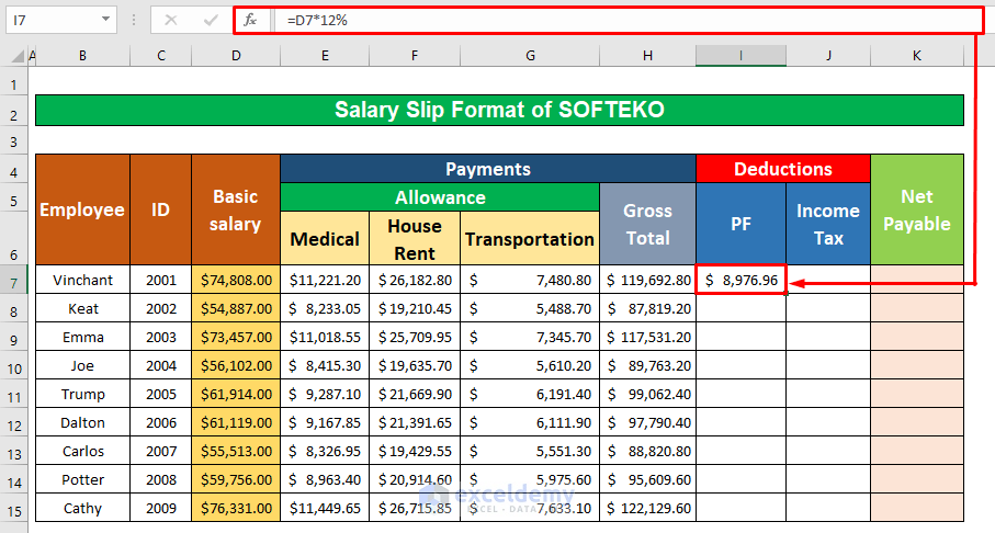
- AutoFill the formula to the rest of the cells in column I.
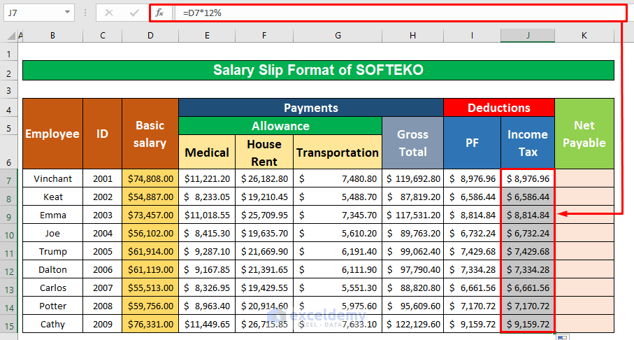
- Calculate the Income Tax in a similar way.
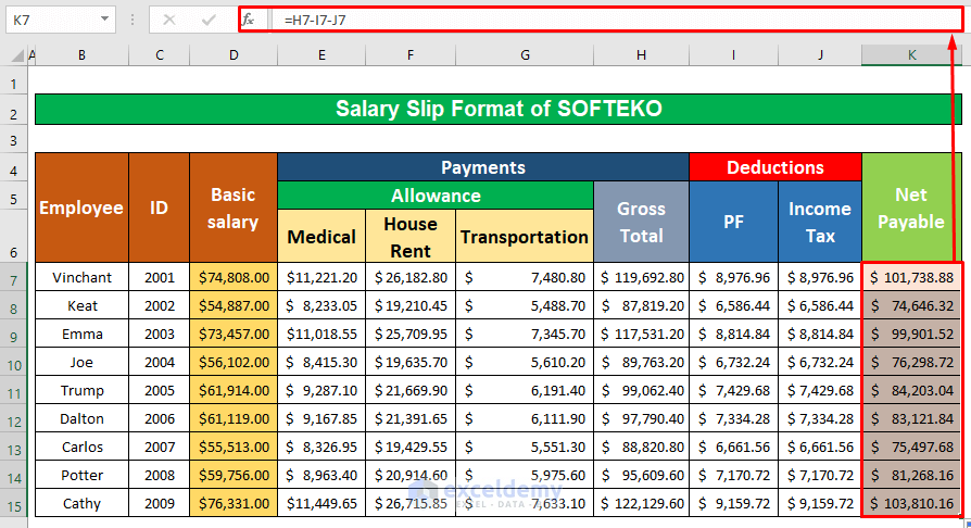
- Copy the following formula in cell K7 to get the Net Payable:
=H7-I7-J7H7 is the Gross total salary, I7 is the Provident Fund balance, and J7 is the Income Tax of the employee.
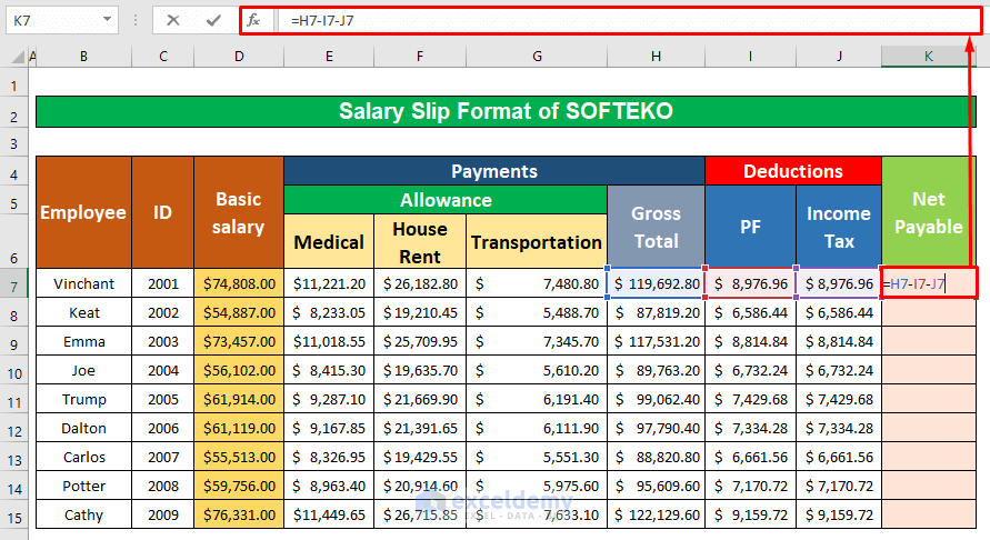
- Hit Enter.
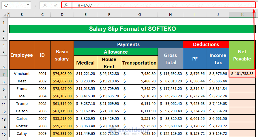
- AutoFill to the rest of the cells in column K.
- This fills the sample dataset.
Download Practice Workbook
Download this practice workbook that you can use as a template. You may need to check with your local laws on the exact values for the taxes and deductions and apply them accordingly.
How to Make Salary Slip in Excel: Knowledge Hub
- How to Create Tally Salary Slip Format in Excel
- Driver Salary Slip Format in Excel
- How to Create Automatic Salary Slip Generator Using Excel
<< Go Back to Salary | Formula List | Learn Excel
Get FREE Advanced Excel Exercises with Solutions!
