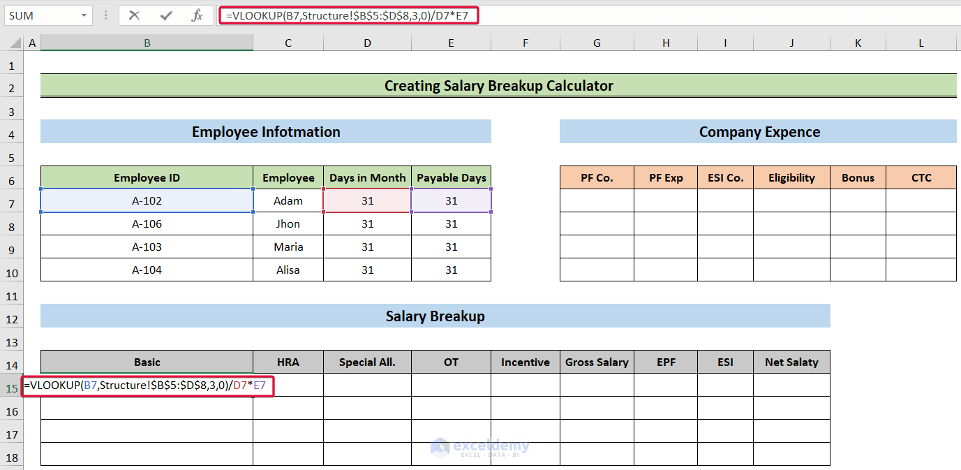
Method 1 – Calculating Basic Salary
- Select the B15 cell and write down the following formula,
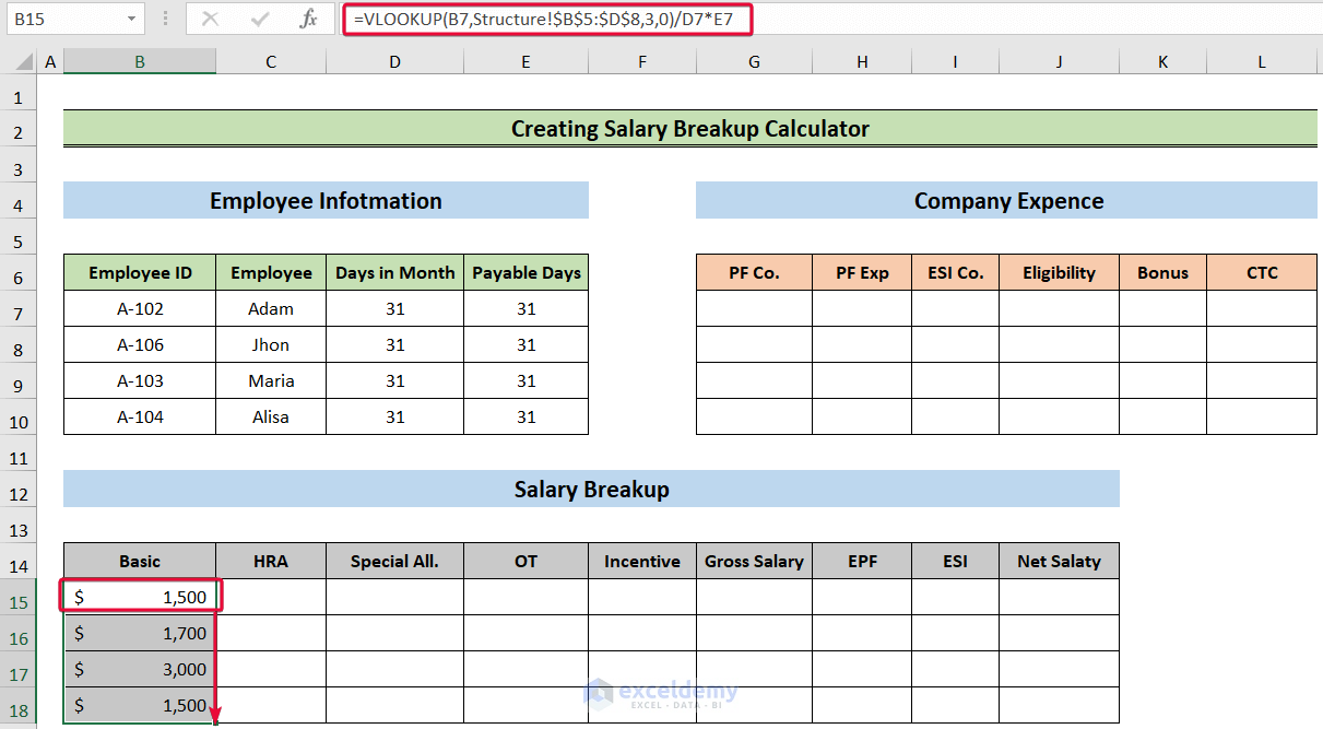
=VLOOKUP(B7,Structure!$B$5:$D$8,3,0)/D7*E7- Hit Enter.
- Have the net basic salary of the employee for that month.
- Move the cursor down to autofill the rest of the cells.
Formula Breakdown:
- VLOOKUP(B7,Structure!$B$5:$D$8,3,0): The VLOOKUP function looks for a value in a range of cells and then returns a value from one of the columns in that range. The VLOOKUP functionlooks for the EmplpyeeID A-102 in the range B5:D8 in the sheet named Structure where we have kept the salary structure of the company. Then, in the 3rd argument we will enter 3 because the value Basic Salary is in the 3rd column of that range. Set the range_lookup value to be zero. So, the function will return $1500 as fits with the employee ID A-102.
- VLOOKUP(B7,Structure!$B$5:$D$8,3,0)/D7*E7: We will try to find out the basic salary to be paid to the employee. It depends on how many days the employee joins the work. The employee has joined all 31 days, so the basic salary will not change as 31 days on the top will nullify 31 days on the bottom.
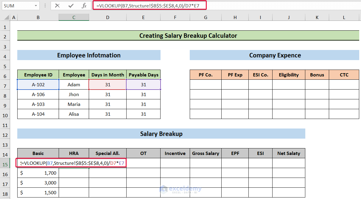
Method 2 – Measuring House Rent Allowance (HRA)
- Select the C15 cell and write the following formula down,
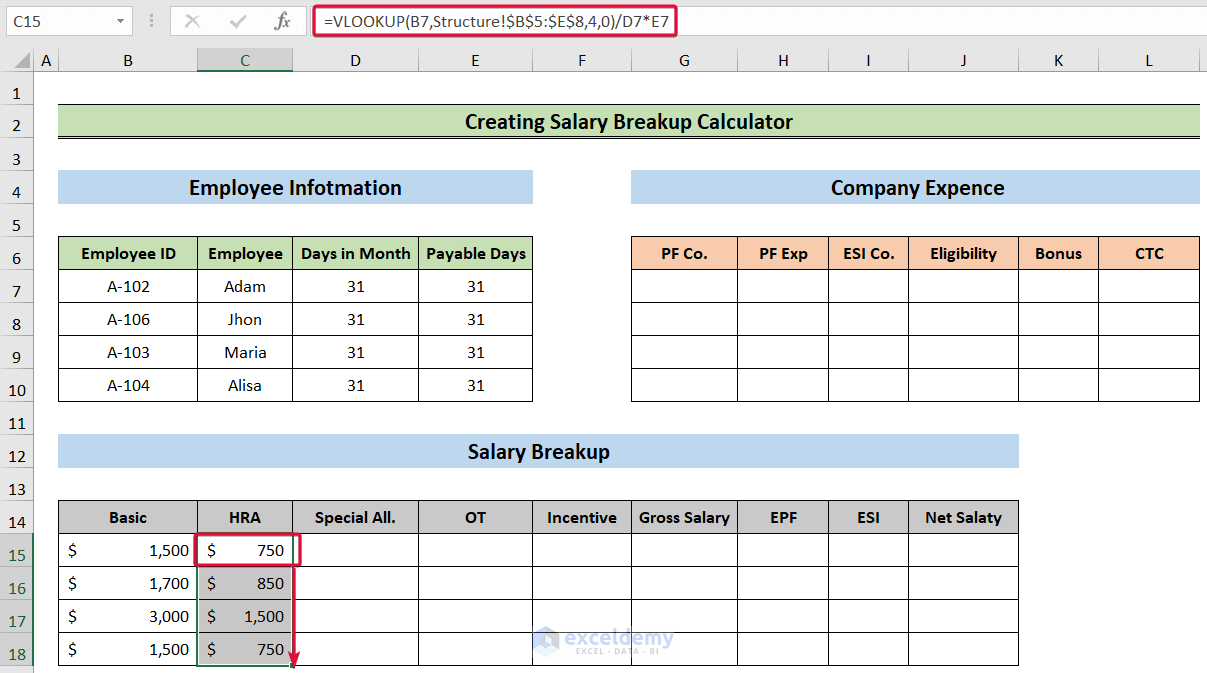
=VLOOKUP(B7,Structure!$B$5:$E$8,4,0)/D7*E7- Hit Enter.
- Have the net HRA of the employee for that month.
- Lower the cursor down to the last cell to autofill.
Method 3 – Calculating Special Allowance
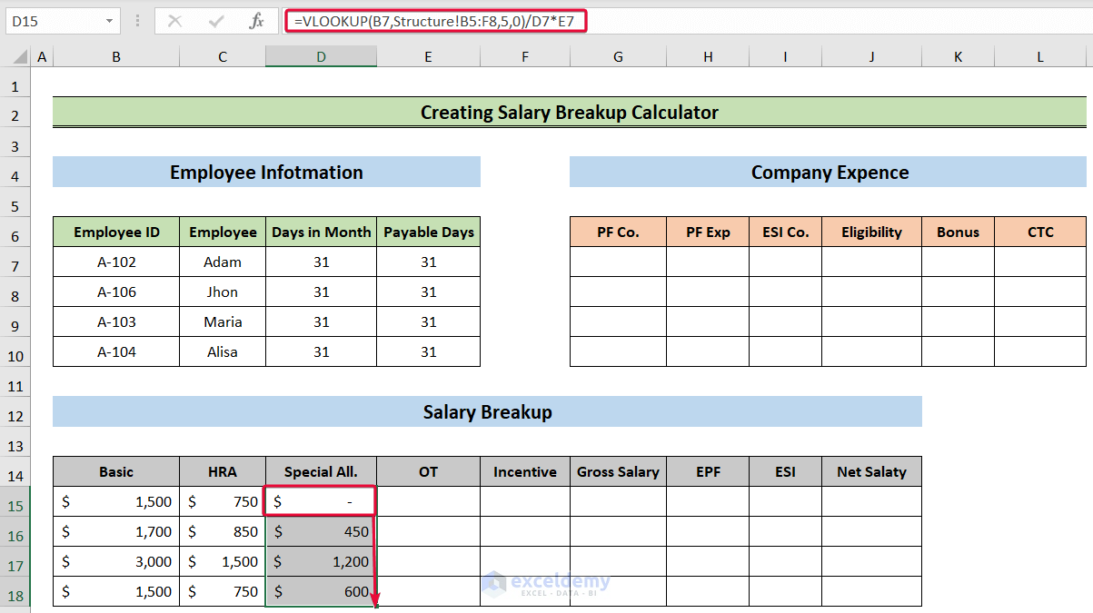
- Choose the D15 cell and type the following,
=VLOOKUP(B7,Structure!B5:F8,5,0)/D7*E7- Press Enter.
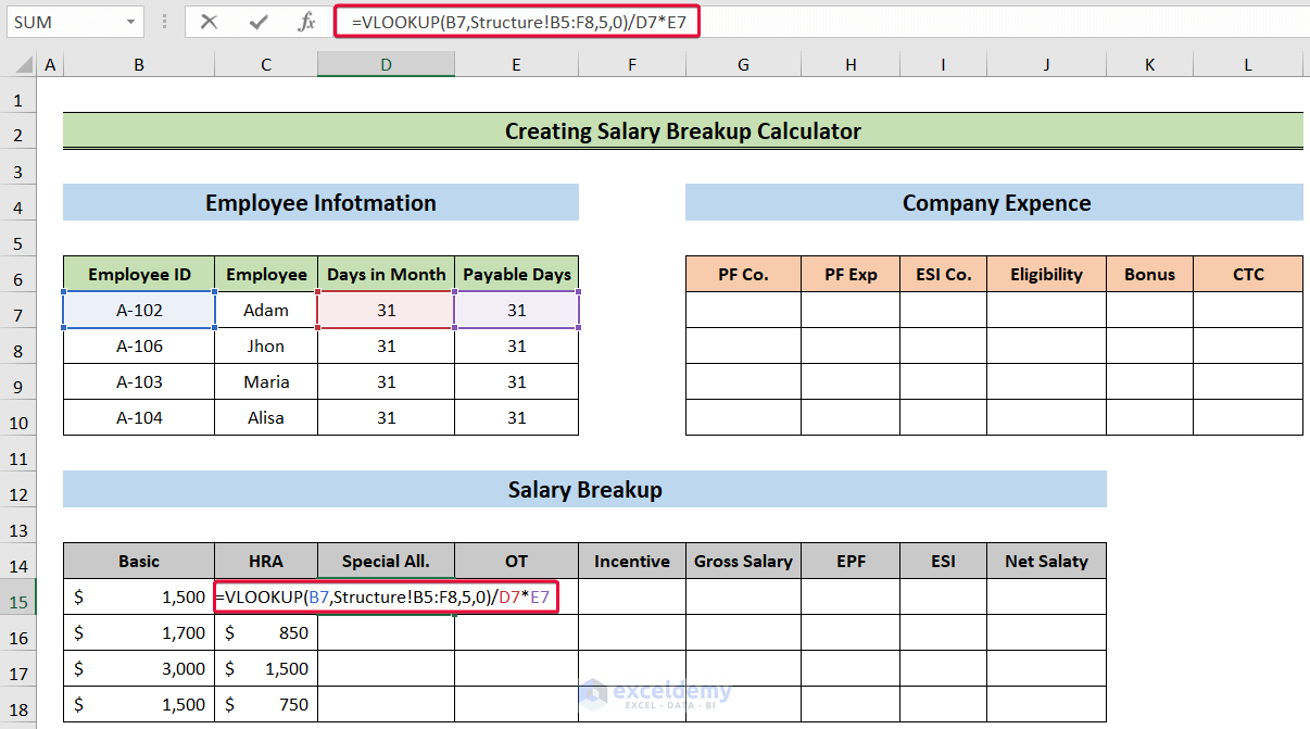
- Get a special allowance for specific employees.
- Move the cursor down to the last cell.
Method 4 – Evaluating Gross Salary
- Choose the G15 cell and write the following,
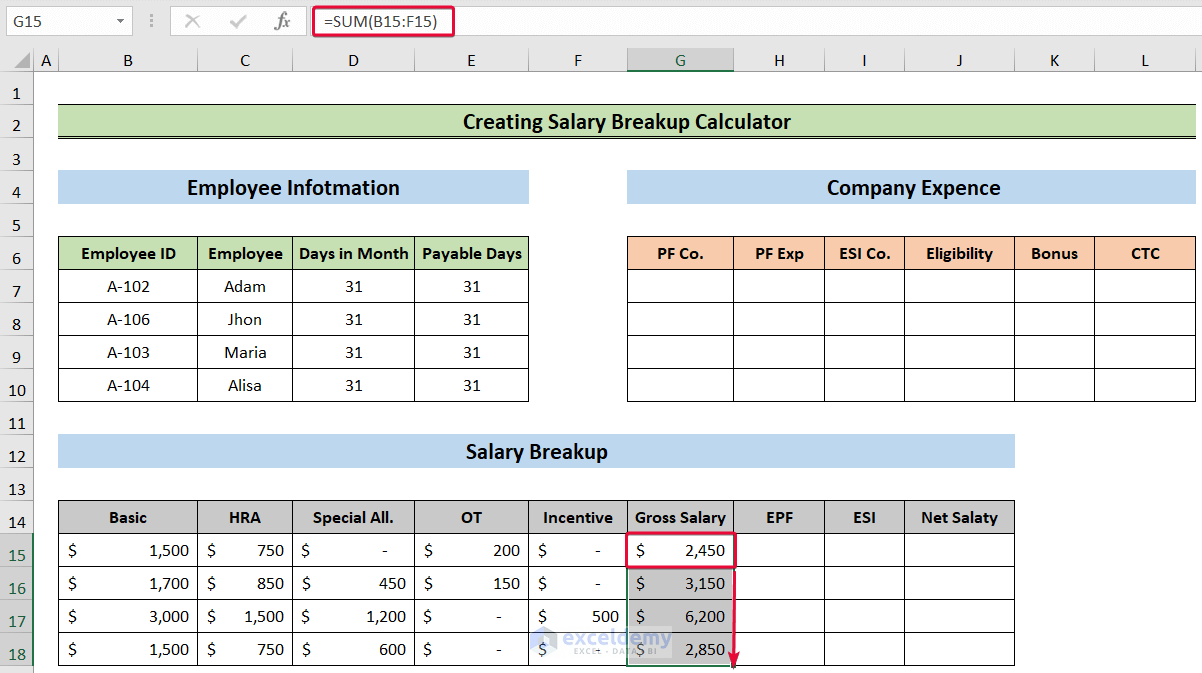
=SUM(B15:F15)- Press Enter.
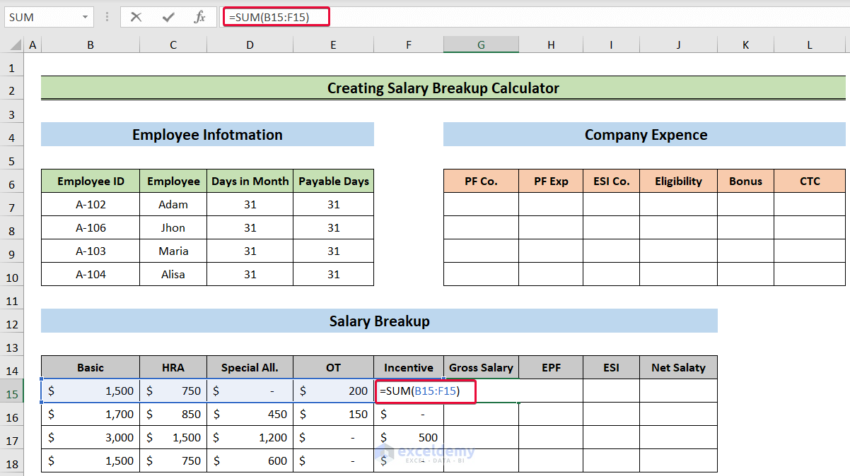
- We will have the gross salary of an employee for that month.
- Lower the cursor down to autofill the rest of the cells.
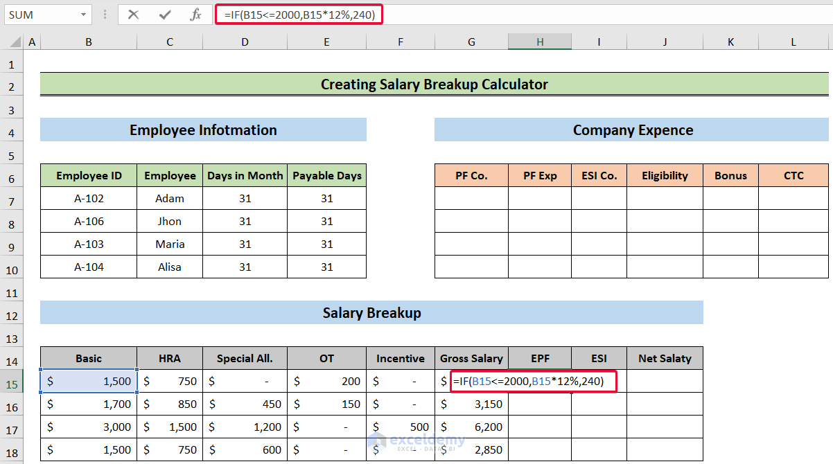
Method 5 – Determining Employees’ Provident Fund (EPF)
- Select the H15 cell and type the following formula,
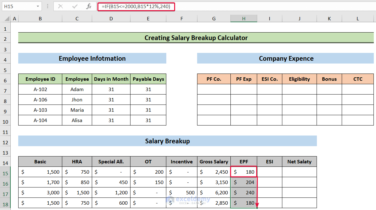
=IF(B15<=2000,B15*12%,240)- Hit Enter.
- Get the EPF amount for that employee.
- Lower the cursor to calculate the EPF for the rest.
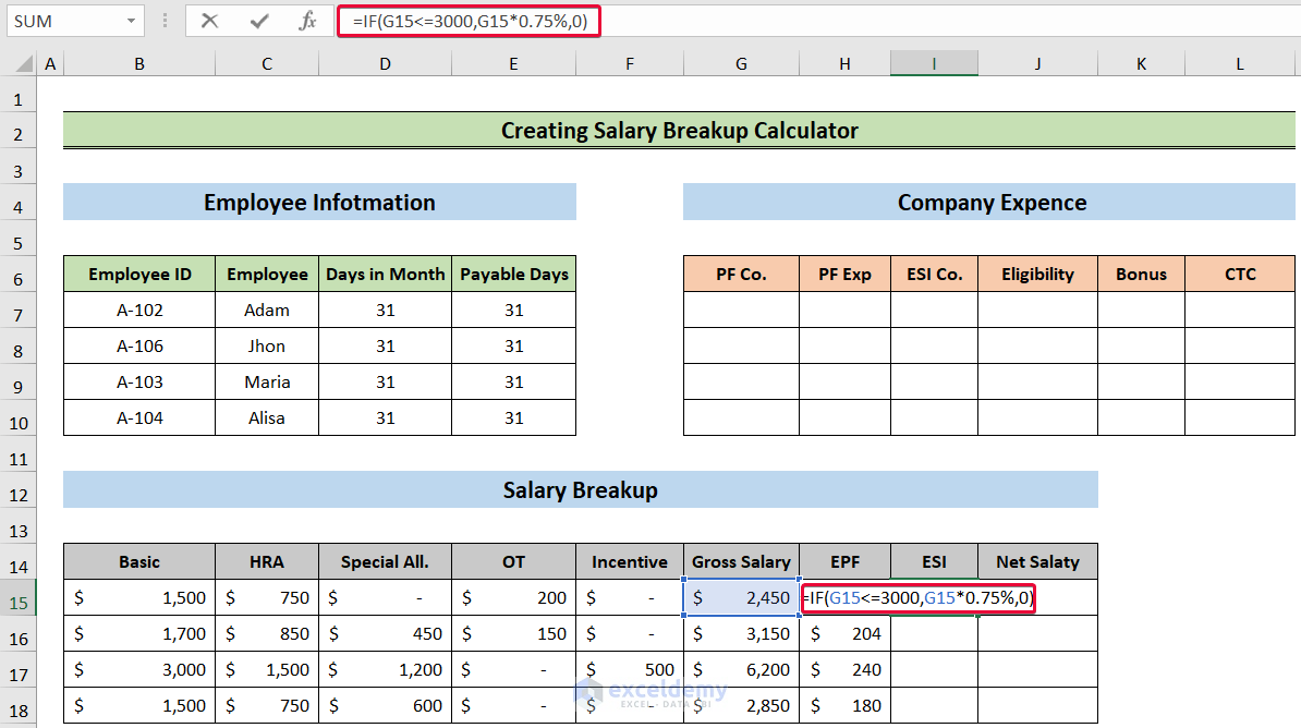
Method 6 – Calculating Employees’ State Insurance Scheme (ESI)
- Select the I15 cell and write down the following,
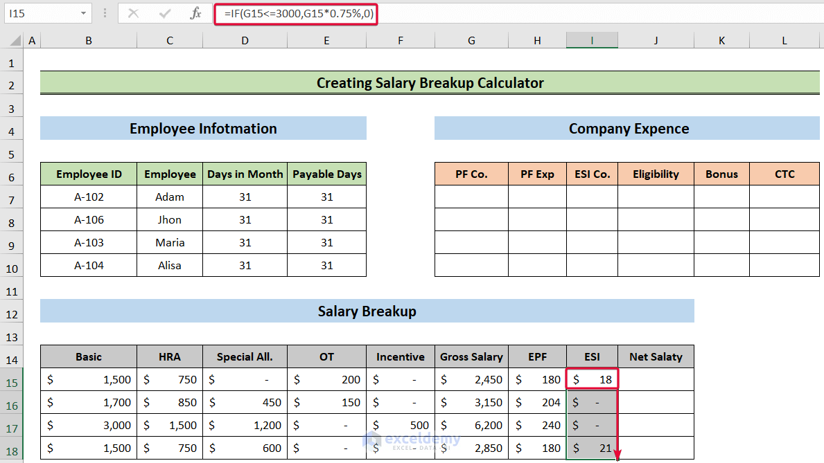
=IF(G15<=3000,G15*0.75%,0)- Hit Enter.
- Have the ESI of the employee for that month.
- Move the cursor down to autofill for the rest of the employees.
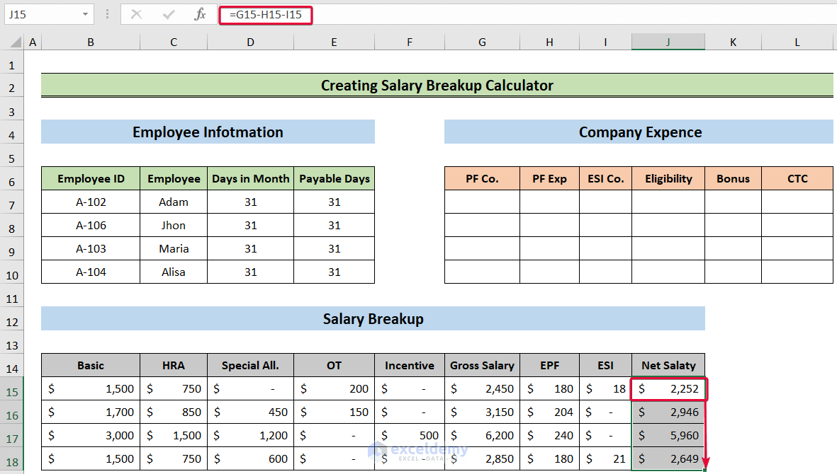
Method 7 – Measuring Net Salary
- Choose the J15 cell and type the following formula in the cell,
=G15-H15-I15- Press Enter.
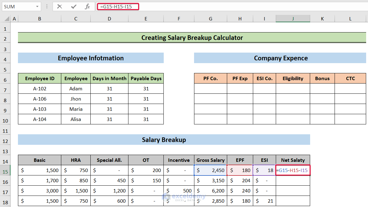
- Get the net salary of the employee.
- Lower the cursor to autofill.
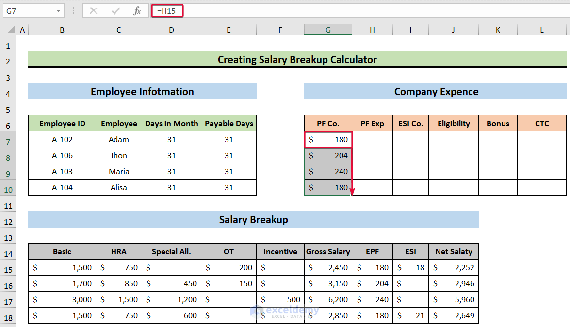
Method 8 – Calculating PF of Company
- Select the G7 cell and write the following in that cell,
=H15- Press Enter.
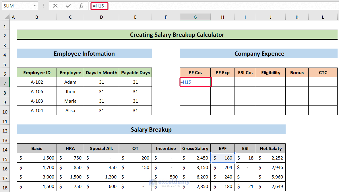
- Get the company’s contribution to the PF.
- Lower the cursor down to autofill the cells.
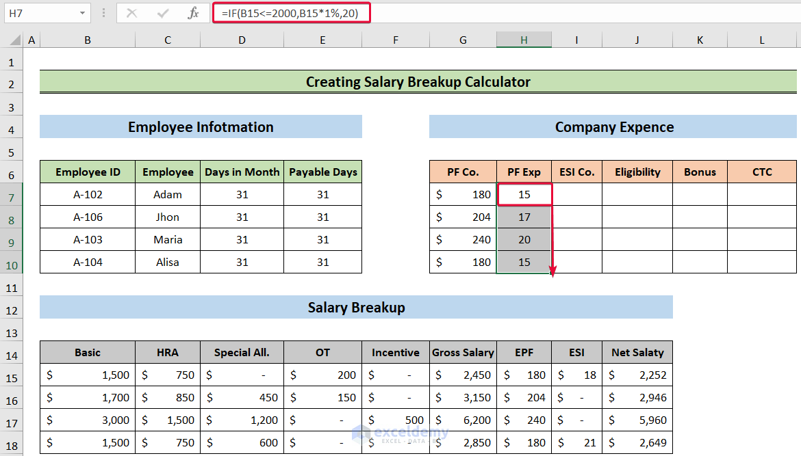
Method 9 – Evaluating PF Expenses
- Start with, choose the H7 cell and type the following formula,
=IF(B15<=2000,B15*1%,20)- Press Enter.
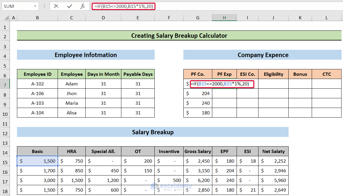
- Get the PF expenses on that employee by the company.
- Move the cursor down to autofill the rest of the cells.
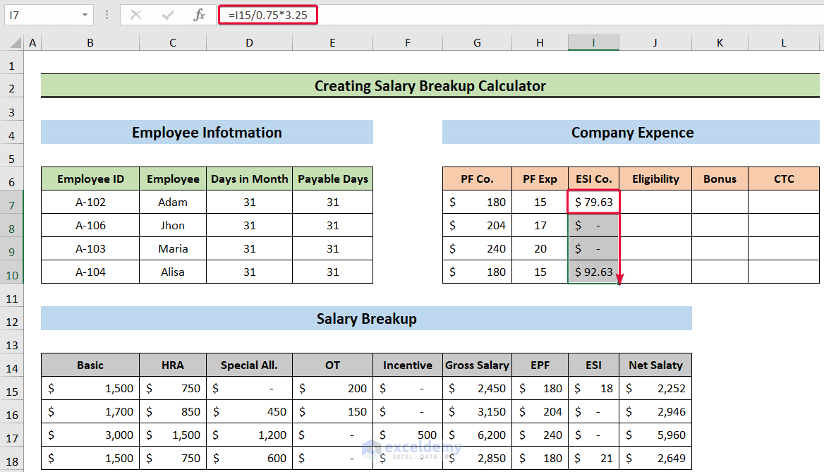
Method 10 – Calculating ESI Company
- Select the I7 cell and write the following in the cell,
=I15/0.75*3.25- Hit Enter.
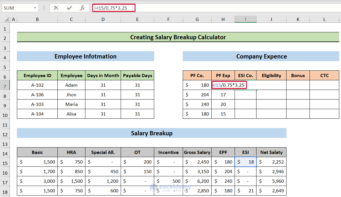
- Get the ESI cost of the company on an employee.
- Lower the cursor down to the last cell.
Method 11 – Measuring Bonus
- Select the K7 cell and type the following,
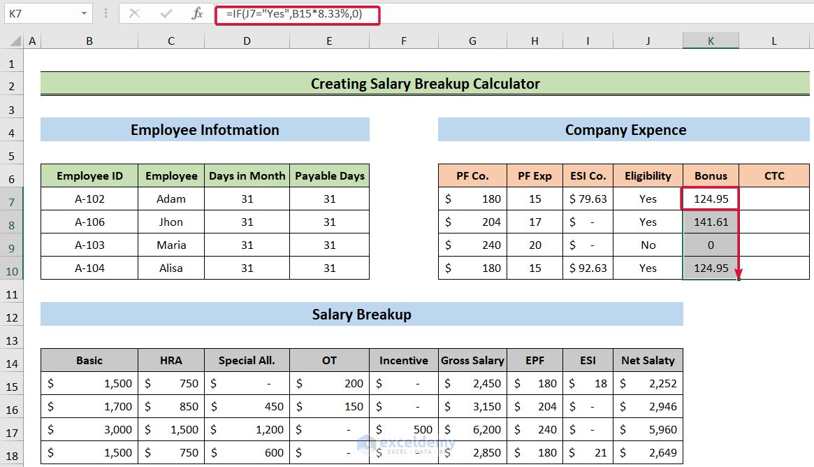
=IF(J7="Yes",B15*8.33%,0)- Press Enter.
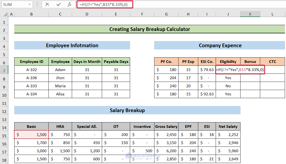
- Get the bonus for that employee (if eligible).
- Lower the cursor down to the last cell.
Method 12 – Calculating CTC
- Select the L7 cell and type the formula below,
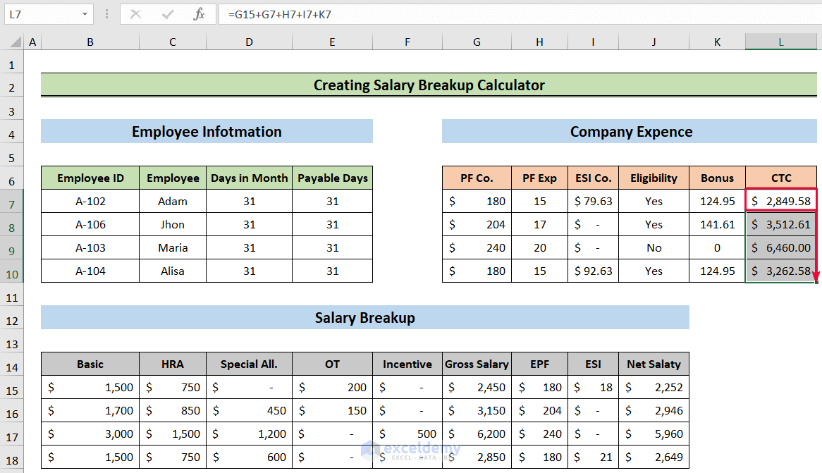
=G15+G7+H7+I7+K7- Hit Enter.
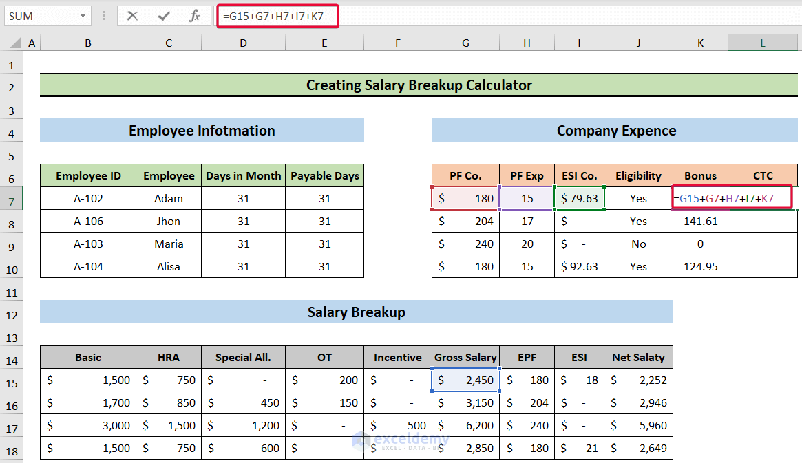
- Get the monthly CTC of an employee.
- Lower the cursor down to autofill the rest of the cells.
Download Practice Workbook
You can download the practice workbook here.
<< Go Back to Salary | Formula List | Learn Excel
Get FREE Advanced Excel Exercises with Solutions!
