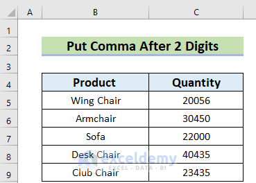
We will use a sample dataset of products and their quantities.
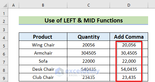
Method 1 – Applying LEFT and MID Functions to Put a Comma After 2 Digits in Excel
Steps:
- Use this formula in the D5 cell.
=LEFT(C5,2)&","&MID(C5,3,10)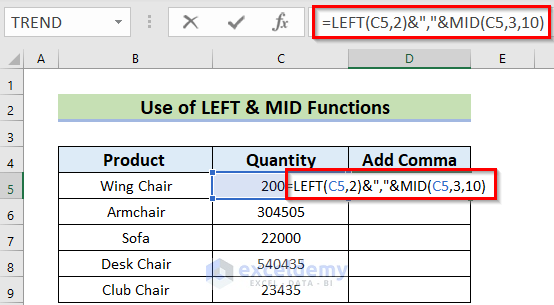
Formula Breakdown
- LEFT(C5,2)—-> The LEFT function will take the leftmost 2 characters from cell C5.
- Output: 20
- The Inverted Comma (“,”) denotes that Comma (,) is a string.
- MID(C5,3,10)—-> The MID function will extract upto 10 characters starting from the 3rd character in cell C5.
- Output: 056
- The Ampersand (&) will join them.
- Output: 20,056
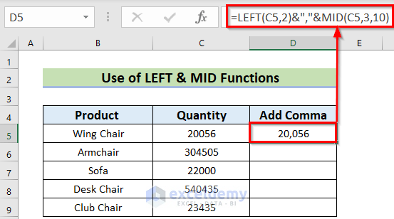
- Hit Enter.
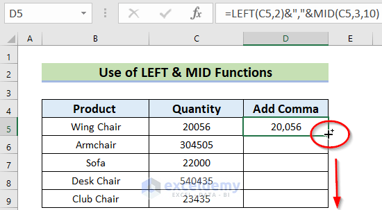
- Drag the Fill Handle icon to AutoFill the corresponding data in the rest of the cells D6:D9.
Here’s the result.
Read More: How to Put Comma in Numbers in Excel
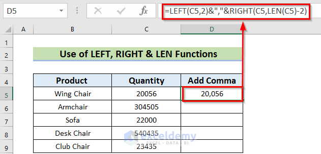
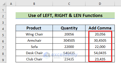
Method 2 – Using the LEFT, RIGHT, and LEN Functions
Steps:
- Use this formula in the D5 cell.
=LEFT(C5,2)&","& RIGHT(C5,LEN(C5)-2)- Hit Enter.
Formula Breakdown
- LEFT(C5,2)—-> The LEFT function will take the leftmost 2 characters from cell C5.
- Output: 20
- LEN(C5)—-> The LEN function will give the total count of the characters in cell C5.
- Output: 5
- RIGHT(C5,5-2)—-> The Right function will take the rightmost 5-2=3 characters of cell C5.
- Output: 056
- The double quotes (“,”) denote that Comma (,) is a string.
- The Ampersand (&) will join them.
- Output: 20,056
- Double-click the Fill Handle icon to AutoFill the corresponding data in the rest of the cells D6:D9.
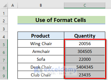
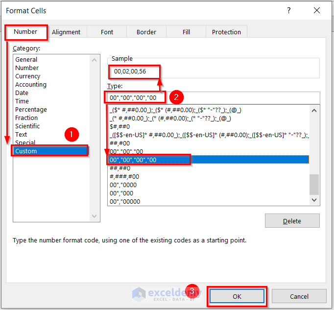
Method 3 – Using the Format Cells Command to Put a Comma After 2 Digits in Excel
Steps:
- Select the range C5:C9.
- Press the Ctrl + 1 keys to open the Format Cells dialog box. Alternatively, go to the Home tab and select the arrow in the Format group.
- Go to the Number tab and select the Custom category.
- Put 00″,”00″,”00″,”00 in the Type option.
- Press OK to get the result.
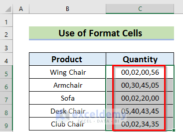
You will see the following result.
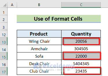
You can use the Format Cells command to put a comma only after 2 digits in Excel. You can follow the steps given below.
- We chose a few cells from the dataset.
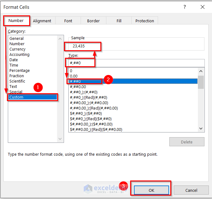
- Open the Format Cells dialog box directly.
- Go to Number and Custom.
- Put #,##0 in the Type option.
This only works on 5-digit numbers.
- Press OK to get the result.
- For cell C14 which has a 6-digit number, use 00″,”0000 in the Type section at the Format Cells dialog box.
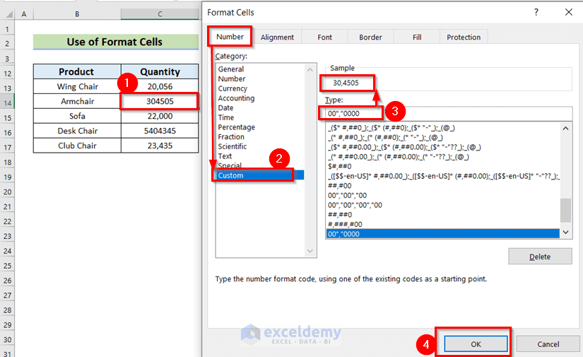
- For cell C16, which has a 7-digit number, use 00″,”00000 in the Type section at the Format Cells dialog box.
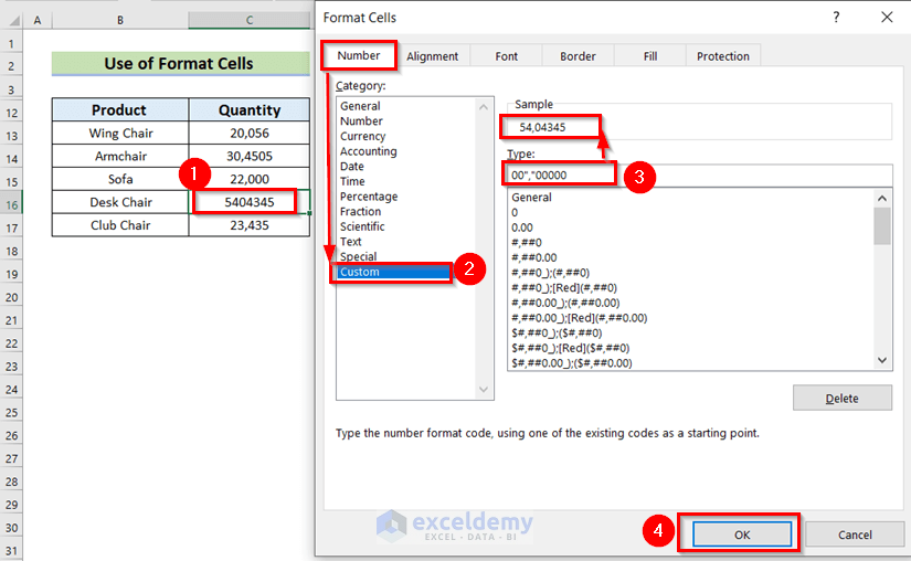
Here are the results.

Read More: How to Put Comma After 5 Digits in Excel
Method 4 – Using the Comma Style Feature
Steps:
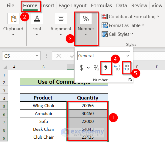
- Select the data range. We have selected C5:C9.
- From the Home tab, go to the Number group.
- Choose Comma Style.
- Click twice on Decrease Decimal to decrease the decimals.
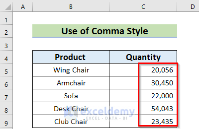
Here are the results.
Read More: How to Change Comma Style in Excel
Method 5 – Applying the Text Function to Put Comma After 2 Digits in Excel
Steps:
- Use this formula in the D5 cell.
=TEXT(C5,"0"",""000")- Hit Enter.
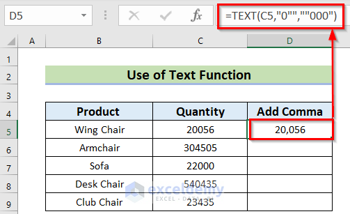
Formula Breakdown
The TEXT function will convert a value to a text and in a certain number format.
- C5 will denote that value.
- The last three zero will count the rightmost 3 characters from the value.
- Output: 056.
- “0””, —> will add the Comma.
- Output: 20,056.
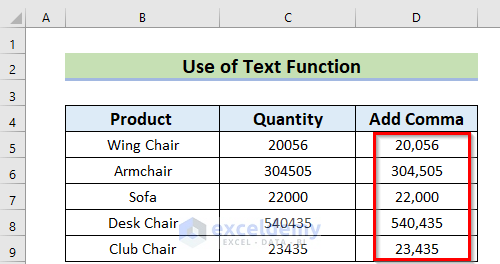
- Double-click the Fill Handle icon to AutoFill the corresponding data in the rest of the cells D6:D9.
- The formula for D6 is:
=TEXT(C6,"0"",""0000")- Here’s the formula for cell D8.
=TEXT(C8,"0"",""0000")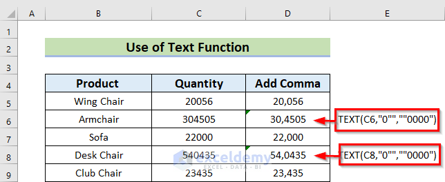
Formula Breakdown
The TEXT function will convert a value to a text including a certain number format.
- C6 will denote that value.
- The last four zero will count the rightmost 4 characters from the value.
- Output: 4505.
- “0””, —> will add the Comma.
- Output: 30,4505.
Here’s the result.

Read More: How to Put Comma after 3 Digits in Excel
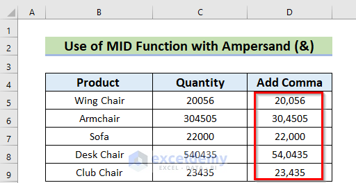
Method 6 – Using the MID Function with the Ampersand Operator
Steps:
- Use this formula in the D5 cell.
=MID(C5,1,2)&","&MID(C5,3,6)- Hit Enter.
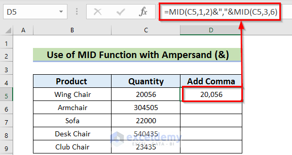
Formula Breakdown
- MID(C5,1,2)—-> The MID function will extract 2 characters starting from the 1st character in cell C5.
- Output: 20
- The double quotes (“,”) denote that Comma (,) is a string.
- MID(C5,3,6)—-> This MID function will extract up to 6 characters starting from the 3rd character in cell C5.
- Output: 056
- The Ampersand (&) will join them.
- Output: 20,056
- Double-click the Fill Handle icon to AutoFill the corresponding data in the rest of the cells D6:D9.
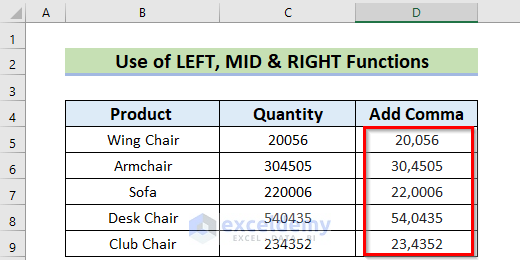
Method 7 – Use Combined Functions to Put a Comma After 2 Digits in Excel
Steps:
- Use this formula in the D5 cell.
=LEFT(C5,2) &","&MID(C5,3,1)& RIGHT(C5,2)- Hit Enter.
Formula Breakdown
- LEFT(C5,2)—-> The LEFT function will take the leftmost 2 characters from cell C5.
- Output: 20
- The double quotes (“,”) denotesthat Comma (,) is a string.
- MID(C5,3,1)—-> The MID function will extract 1 character starting from the 3rd character in cell C5.
- Output: 0
- RIGHT(C5,2)—-> The RIGHT function will take the rightmost 2 characters of cell C5.
- Output: 56
- The Ampersand (&) will join them.
- Output: 20,056
- For a 6-digit number, you should use the following formula in cell D6.
=LEFT(C6,2) &","&MID(C6,3,2)& RIGHT(C6,2)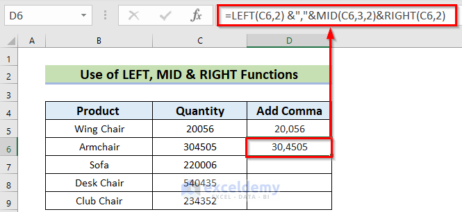
Formula Breakdown
- LEFT(C6,2)—-> The LEFT function will take the leftmost 2 characters from cell C6.
- Output: 30
- The double quotes (“,”) denote that Comma (,) is a string.
- MID(C6,3,2)—-> The MID function will extract 2 characters starting from the 3rd character in cell C6.
- Output: 45
- RIGHT(C6,2)—-> The RIGHT function will take the rightmost 2 characters of cell C6.
- Output: 05
- The Ampersand (&) will join them.
- Output: 30,4505
- Double-click the Fill Handle icon to AutoFill the corresponding data in the rest of the cells D7:D9. Those cells contain 6-digit numbers.
Method 8 – Applying the Currency Feature
Steps:
- Select the data range.
- From the Home tab, go to the Number group.
- Click on the Drop-Down box and choose Currency.
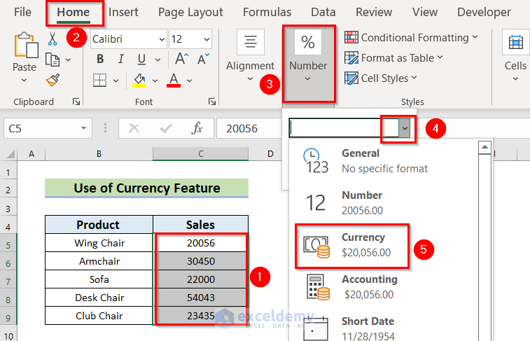
- Click two times on Decrease Decimal to decrease the decimal.
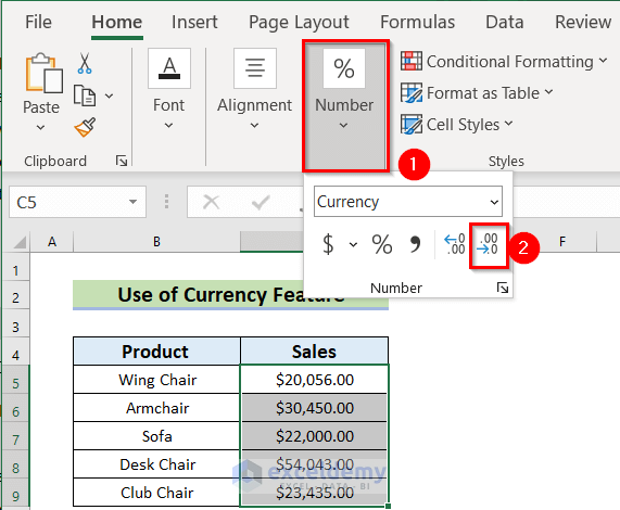
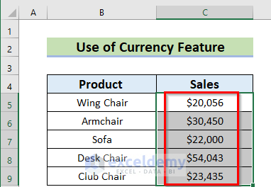
Here’s the result.
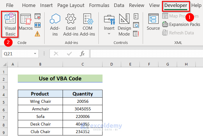
Method 9 – Using VBA Code to Put a Comma After 2 Digits in Excel
Steps:
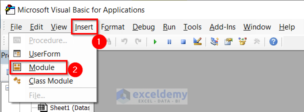
- Choose the Developer tab and select Visual Basic.
- From the Insert tab, select Module.
- Use the following Code in the Module.
Sub AddComma()
Dim data_range As Range
Dim digit1 As Long
Dim digit2 As Long
Dim num As String
Dim digit3 As Long
Application.ScreenUpdating = False
For Each data_range In Selection
If IsNumeric(data_range.Value) Then
If data_range.Value < 0 Then
digit3 = 2
Else
digit3 = 1
End If
digit2 = Len(data_range.Value)
num = ""
For digit1 = digit2 - 2 To digit3 Step -2
num = """,""00" & num
Next digit1
If digit2 Mod 2 Or digit3 = 2 Then
num = "00" & num
Else
num = "00" & num
End If
data_range.NumberFormat = num
End If
Next data_range
Application.ScreenUpdating = True
End Sub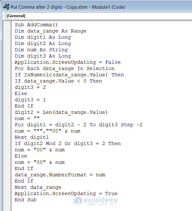
Code Breakdown
- We have created a Sub Procedure named AddComma.
- We declared some variables data_range as Range to call the range; digit1 as Long; digit2 as Long; num as String; digit3 as Long.
- The Selection property will select the range from the sheet.
- We used a For Each Loop to put Comma in each selected cell using a VBA If function to do a logical test.
- Save the code and go back to the Excel File.
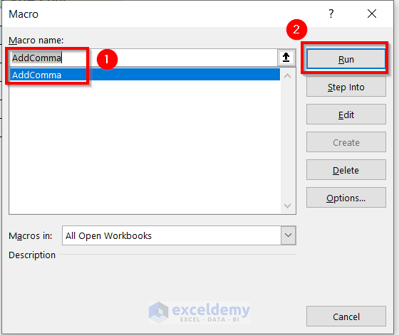
- Select the range C5:C9.
- From the Developer tab, select Macros.
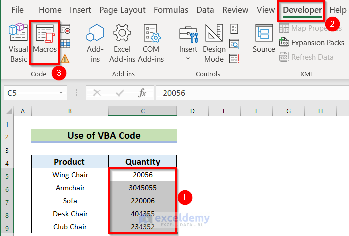
- Select AddComma and click on Run.
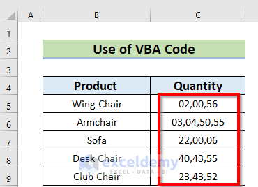
You will see the following result.
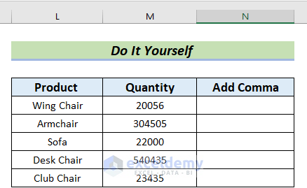
Practice Section
You can use the sample dataset to test these methods.
Download the Practice Workbook
Related Articles
- How to Convert Column to Row with Comma in Excel
- How to Change Semicolon to Comma in Excel
- How to Change Comma in Excel to Indian Style
- [Fixed!] Style Comma Not Found in Excel
<< Go Back to How to Add Comma in Excel | Concatenate Excel | Learn Excel
Get FREE Advanced Excel Exercises with Solutions!
