How to Multiply Time by Money in Excel (with Easy Steps)

Get FREE Advanced Excel Exercises with Solutions!

The managers in a company often find it difficult to multiply time by the rate of money to get the total daily payment. This can be easily done in Excel. But most managers find it onerous to multiply time by money in Excel. Thus, they can not keep track of the total salary of the employees. Manual tracking only makes their lives harder. For this reason, in this article, we will discuss in detail how to multiply time by money in Excel.

Table of Contents hide

Download the Practice Workbook

Step-by-Step Procedures to Multiply Time by Money in Excel

Step 1: Calculating Time Difference

Step 2: Changing Data Format

Step 3: Displaying Time Difference in Fraction

Step 4: Changing Fractional Times

Step 5: Applying Conditions to Hourly Pay Rate

Step 6: Using IF Function

Step 7: Multiply Time by Money

Conclusion

Download the Practice Workbook

Multiply Time by Money.xlsx

Step-by-Step Procedures to Multiply Time by Money in Excel

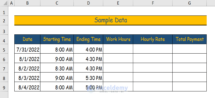
In this Excel tutorial, we will discuss how to multiply time by money. Here, we will talk about the formulas that will allow us to multiply time by money in Excel. We will also use the IF Function to make the example more pragmatic. We will explain each steps to multiply time by money in Excel. We will use the sample data below to illustrate the procedures.

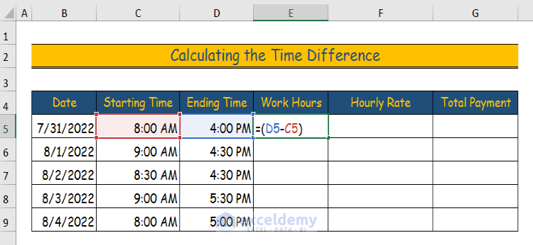
Step 1: Calculating Time Difference

Firstly, select the first cell under the “Work Hour”.
In our case, we will select the E5 cell.
Then, type the equal sign to enter the formula below.

=(D5-C5)

In this formula, we will subtract “Starting Time” from “Ending Time”.
In this instance, we will take the C5 cell out of the D5 cell.
Then, hit Enter.

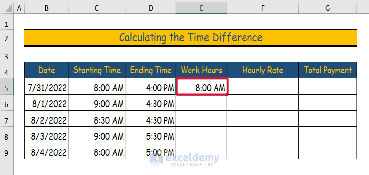
As a result, you will notice that a time has been added to that cell.
It is because the number in the cell is formatted for Time format.

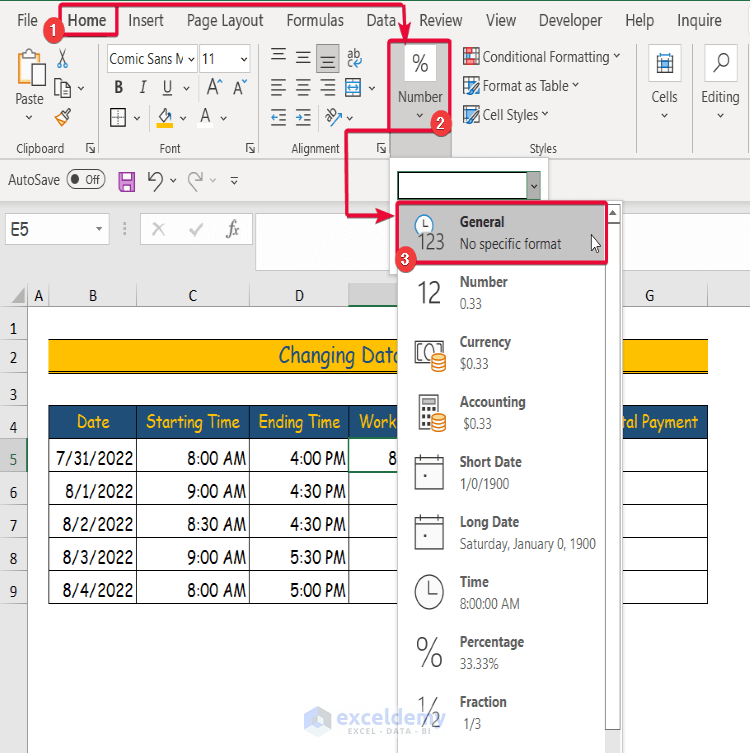
Step 2: Changing Data Format

Secondly, go to the Home tab.
Then, navigate to the Number group.
From the box in the Number group, make the number type from Time to General.

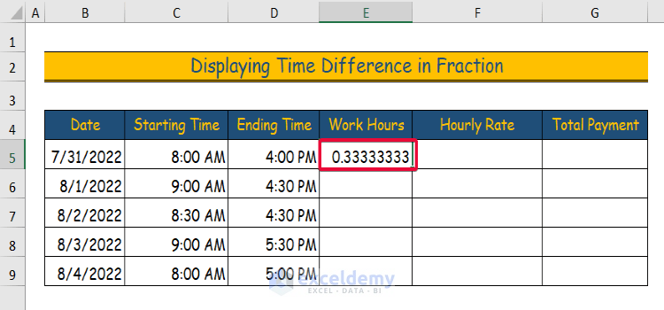
Step 3: Displaying Time Difference in Fraction

Consequently, you will see that the cell shows a fraction.
In this case, cell E5 shows 0.33333333.
This is because Excel saves time as a fraction of 24 hours.

Similar Readings

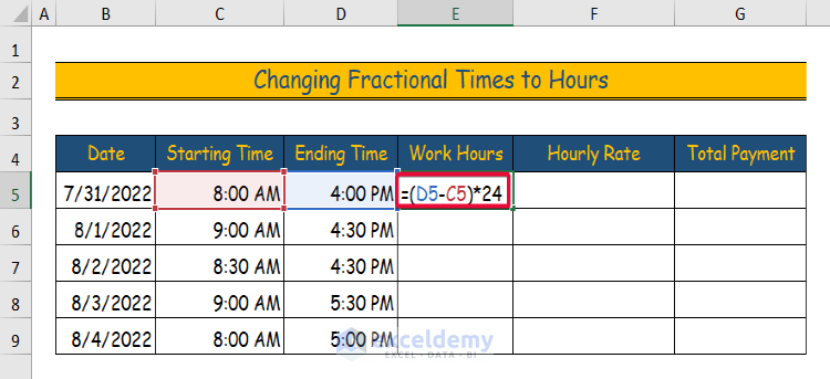
Step 4: Changing Fractional Times

Thirdly, you will multiply the cell by 24.
Write the following formula,

=(D5-C5)*24

In our example, we will multiply the value in the E5 which is (D5-C5) cell by 24.
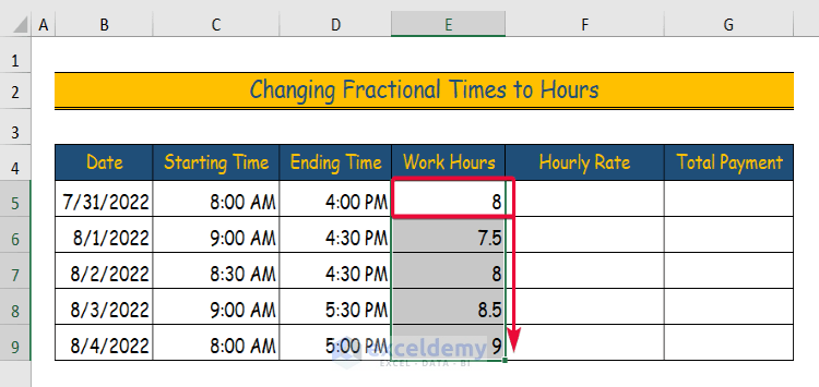
As a result, the cell will show the desired time difference.
In our case, it is 8.

After that, we will move the cursor down to the last cell of the dataset.
Excel will automatically complete the rest of the values.

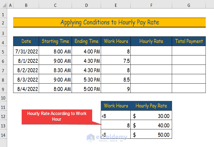
Step 5: Applying Conditions to Hourly Pay Rate

The amount paid per hour depends on how many hours the employee has put in.
In our case, we will indicate the rates as follows.

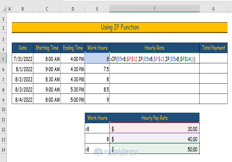
Step 6: Using IF Function

Now, select the first cell under the “Hourly Rate”
In this case, we will go for the F5 cell.
Then, type equal and write this formula below,

=IF(E5<8,$F$12,IF(E5=8,$F$13,IF(E5>8,$F$14)))

Finally, hit Enter.

Formula Breakdown

IF(E5>8,$F$14): This is the IF formula which takes 3 arguments, namely:logical_test, value_if_true,value_if_false. The logical_test argument seeks the data on which it will imply the condition. In our case, the cell with the data is E5 and the condition is if the value in the E5 cell is greater than 8. The argument value_if_true adds the value to the cell if the condition is satisfied. In our case, the value is $50.
IF(E5=8,$F$13,IF(E5>8,$F$14)): This is a nested if statement, which means it has an f statement inside of another if statement. Here, the value_if_false argument of the first if statement is the second if statement. In other words, if the value in the cell does not satisfy the condition in the first if statement then it will go to the second if statement. Here, the first condition is if the value in E5 is equal to 8. If it is true, then Excel will assign the value in the F13 cell to the E5 cell, which is $40.
IF(E5<8,$F$12,IF(E5=8,$F$13,IF(E5>8,$F$14))): This is another nested if statement. Here too, the value_if_false argument of the first if statement is the second if statement. In other words, the second if statement will be invoked if the value in the cell does not meet the criteria in the first if statement. Here, the first condition is if the value in E5 is less than 8. If it is true, then Excel will assign the value in the F12 cell to the E5 cell which is $30.

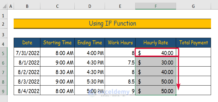
Consequently, the cell will contain a value according to the conditions.
Then, slide the cursor down to the last cell of the dataset.
Excel will automatically fill the rest of the cells.

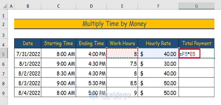
Step 7: Multiply Time by Money

After that, go to the first cell under the “Total Payment”
Here, we choose cell G5.
Then, type the equal sign followed by the following formula,

=F5*E5

Here, we will multiply the corresponding value in the “Work Hour” cell by the “Hourly Rate” cell value.
In this example, we will multiply cell F5 by cell E5.
Finally, hit Enter.

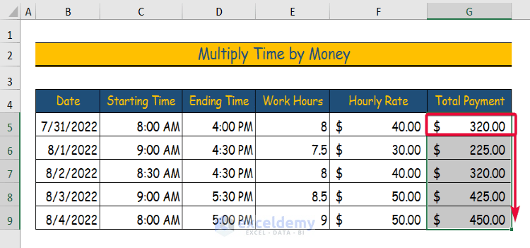
Consequently, we will get our desired total payment.
After that, lower the cursor to the final data cell.
Excel will auto-fill The rest of the cells.

Conclusion

In this article, we have discussed the procedures to multiply time by money. After going through this article, Excel users will have a clear understanding of how the time variables are stored in Excel. This will allow them to multiply time by money and keep track of the total payment for a certain number of work hours. If you find it useful, please let us know in the comment section below and share any recommendations and thoughts regarding this or any other content of ours. Thank you for your time. Follow ExcelDemy.com for more articles like this.

How to Multiply Time by Money in Excel (with Easy Steps)

Download the Practice Workbook