How to Calculate Cash Flow in Excel (8 Examples)

Below is a dataset with 5 Rows: Discount Rate, Year, Investing CF, Financing CF, and Operating CF.

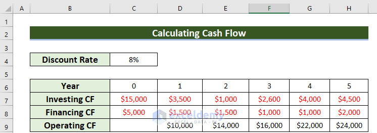
Investing Cash Flow and Financing Cash Flow denote the cash outflows for a business that have negative values (in red).

Method 1 – Using the NPV Function

Steps:

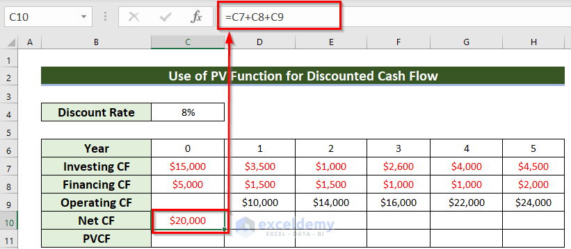
Select a cell, C10, where you want to see the Net CF.
Enter the following formula in cell C10:

=C7+C8+C9

Press ENTER.

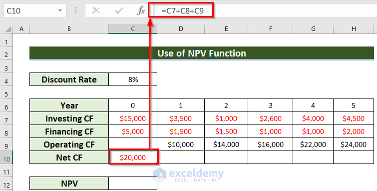
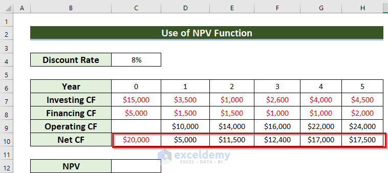
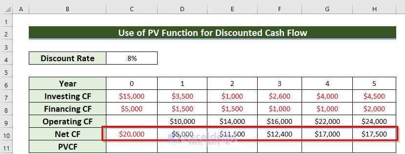
Drag the Fill Handle icon horizontally to AutoFill the data in the rest of the cells D10:H10.

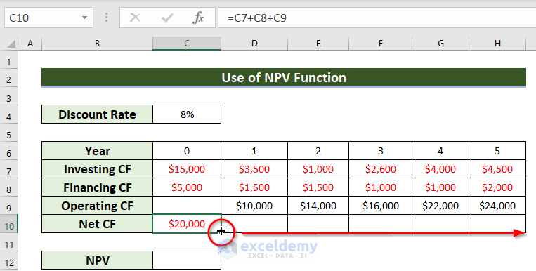
You can see the Net Cash Flow for all those given periods.

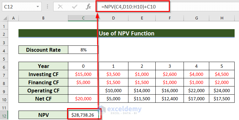
Select a cell, C12, where you want to keep the Net Present Value.
Enter the following formula in cell C12:

=NPV(C4,D10:H10)+C10

Press ENTER to get the result.

You will get the Net present value of Cash flow.

Formula Breakdown

The NPV function will return the Net present value based on a discount rate, cash inflows, and cash outflows of an investment.

C4 is the Discount Rate.
The data range D10:H10 denotes the cash flows.
NPV(C4,D10:H10)—> becomes $48,738.26.
I have included the total outflows of the beginning year. As C10 is the outflow amount of the initial year, thus, I have added the value of the C10 cell.
So, $48,738.26+(-$20,000)—> turns $28,738.26.

Method 2 – Employing PV Function

Steps:

Select a cell, C10, where you want to see the Net CF.
Enter the following formula in cell C10:

=C7+C8+C9

Press ENTER to get the result.

Drag the Fill Handle icon horizontally to AutoFill the data in the rest of the cells D10:H10.

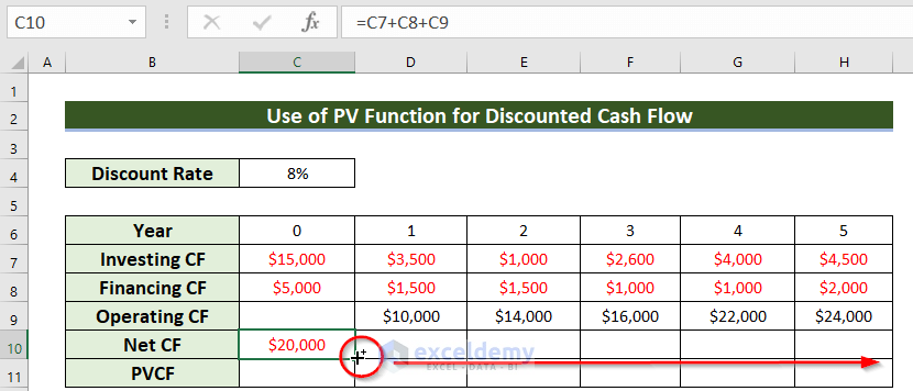
You will get the Net Cash Flow.

Select a cell, C11, where you want to keep the Present Value.
Enter the following formula in cell C11:

=PV($C$4,C6,0,C10)

Press ENTER to get the result.

You will get the Present value of Cash flow.

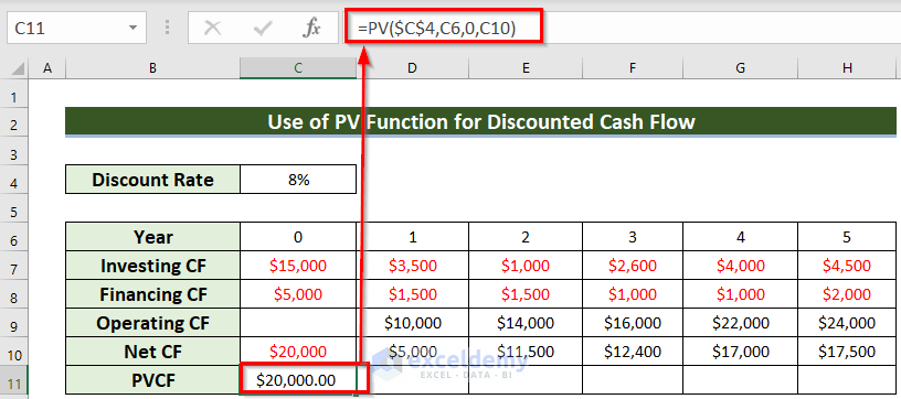
Formula Breakdown

Here, the PV function will return the Present Value of an investment.

$C$4 denotes the discount rate. Here, the Dollar sign ($) denotes that the value is fixed.
C6 denotes NPER as the period of time.
0 denotes that you don’t know the PMT.
C10 denotes the Net Cash flow as Future Value.

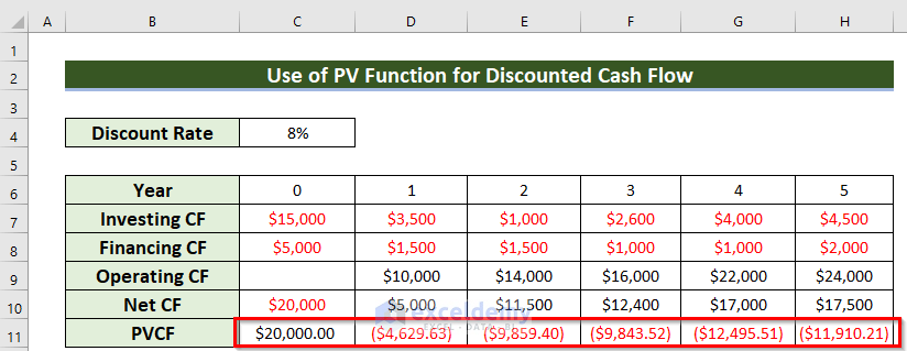
Drag the Fill Handle icon horizontally to AutoFill the data in the rest of the cells D11:H11.

You will get all the Present value of the Cash flow.

Method 3 – Using a Generic Formula

Steps:

Select a cell, C10, where you want to keep the PV factor.
Enter the following formula in cell C10.

=1/(1+$C$4)^C6

Press ENTER to get the result.

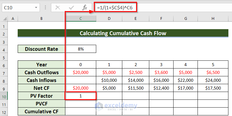
Formula Breakdown

Here, I have added 1 with the discount rate.
- 1+$C$4—> becomes 108%.
I have kept the Year as the power function.
- 108%^C6—> turns 1.
I have divided 1 by the previous output.
- 1/1—> returns 1.

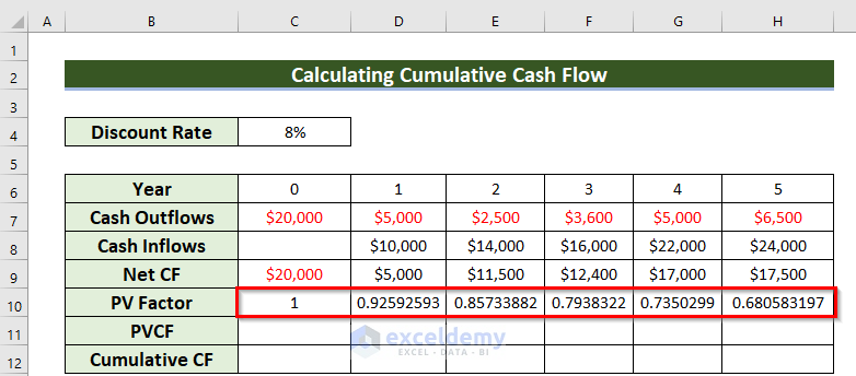
Drag the Fill Handle icon horizontally to AutoFill the data in the rest of the cells D10:H10.

You will get all the Present value factors.

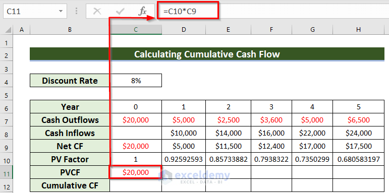
Select a cell, C11, where you want to keep the Present Value.
Enter the following formula in the C11 cell.

=C10*C9

In this formula, I have multiplied the PV factor with the Net Cash flow.

Press ENTER to get the result.

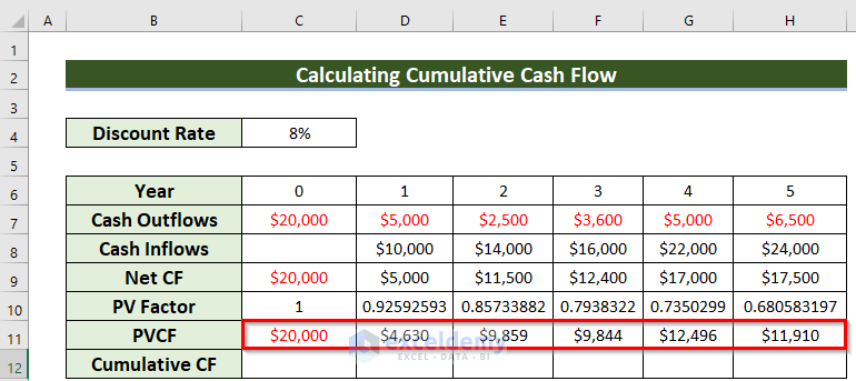
You will get the present value of Cash flow.

Drag the Fill Handle icon horizontally to AutoFill the data in the rest of the cells D11:H11.

You will get all the Present value cash flow.

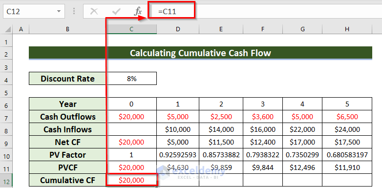
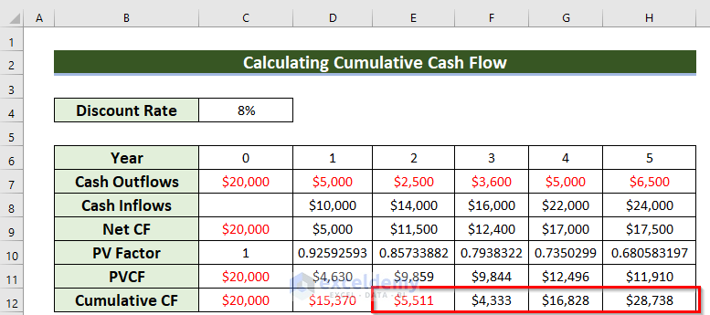
Enter the following formula in cell C12:

=C11

In this formula, I have used the value of the C11 cell.

Press ENTER to get the result.

You will get the 1st Cumulative Cash flow.

Enter the following formula in cell D12:

=C12+D11

Press ENTER to get the result.

This is the 2nd Cumulative Cash flow.

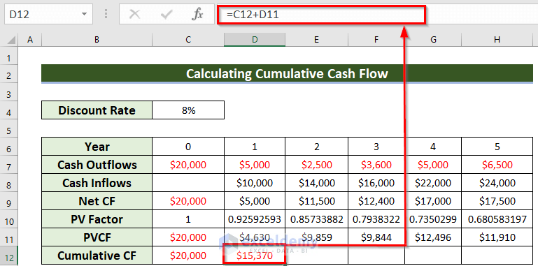
Drag the Fill Handle icon horizontally to AutoFill the data in the rest of the cells E12:H12.

You will get all the Cumulative Cash flow for the given periods.

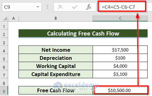
Method 4 – Calculating Free Cash Flow

Steps:

Select a cell, C9, where you want to keep the Free Cash Flow.
Enter the following formula in cell C9:

=C4+C5-C6-C7

In this formula, I have added Net income and Depreciation. From that added value, I have subtracted Working capital and Capital expenditures.

Press ENTER to get the result.

You will get the Free Cash Flow.

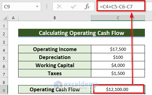
Method 5 – Calculating Operating Cash Flow

Steps:

Select a cell, C9, where you want to keep the Operating Cash Flow.
Enter the following formula in cell C9:

=C4+C5-C6-C7

In this formula, I have added Operating income and Depreciation. From that added value, I have subtracted Working capital and Taxes.

Press ENTER to get the result.

You will get the Operating Cash Flow.

Method 6 – Calculating Cash Flow Forecast

Steps:

Select a cell, C8, where you want to keep the Cash Flow Forecast.
Enter the following formula in cell C8:

=C4+C5-C6

In this formula, I have added the Beginning Cash and Project Inflows. And, from that added value I have subtracted Project Outflows.

Press ENTER to get the result.

You will get the Cash Flow Forecast.

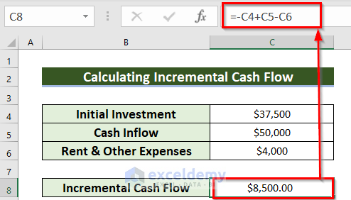
Method 7 – Finding Incremental Cash Flow

Steps:

Select a cell, C8, where you want to keep the Incremental Cash flow.
Enter the following formula in cell C8:

=-C4+C5-C6

In this formula, I have subtracted Initial Investment and Rent & Other expenses from the total Cash Inflow.

Press ENTER to get the result.

You will get the Incremental Cash flow.

Method 8 – Calculating Internal Return Rate

Steps:

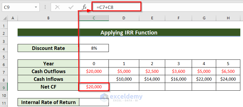
Select a cell, C9, where you want to see the Net CF.
Enter the following formula in cell C9:

=C7+C8

In this formula, I have added all the cash flows to find the net cash flow.

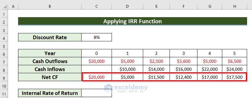
Press ENTER to get the result.

Drag the Fill Handle icon horizontally to AutoFill the data in the rest of the cells D9:H9.

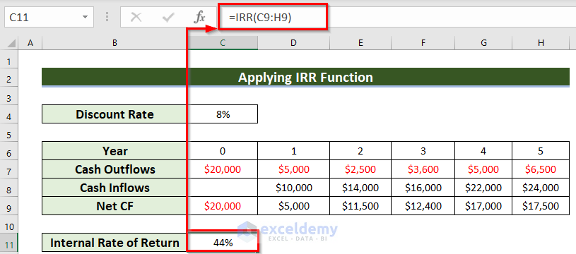
Select another cell, C11, to keep the Internal Rate of Return.
Enter the following formula in cell C11:

=IRR(C9:H9)

Here, C9:H9 is the data range for the IRR function.

Press ENTER to get the result.

You will get the Internal Rate of Return for the Cash flow.

Things to Remember

Here, you must use the negative sign for all the Cash outflows. Otherwise, you have to modify all those given formulas. But, in the case of examples 4 to 7 you don’t need to use minus sign as input.

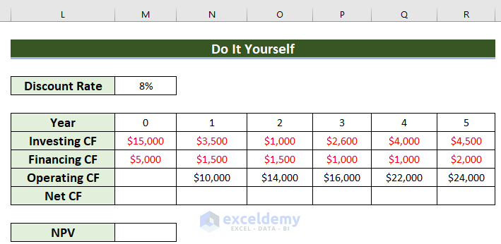
Practice Section

Now, you can practice.

Download the Practice Workbook

You can download the practice workbook from here:

Calculating Cash Flow.xlsx

Excel Cash Flow Formula: Knowledge Hub

<< Go Back to Excel Formulas for Finance | Excel for Finance | Learn Excel

Get FREE Advanced Excel Exercises with Solutions!

How to Calculate Cash Flow in Excel (8 Examples)

Method 1 – Using the NPV Function

Method 2 – Employing PV Function

Method 3 – Using a Generic Formula

Method 4 – Calculating Free Cash Flow

Method 5 – Calculating Operating Cash Flow

Method 6 – Calculating Cash Flow Forecast

Method 7 – Finding Incremental Cash Flow

Method 8 – Calculating Internal Return Rate

Things to Remember

Practice Section

Excel Cash Flow Formula: Knowledge Hub

Leave a reply Cancel reply