How to Calculate Payback Period in Excel (With Easy Steps)

Step 1 – Calculating Net Cash Flow

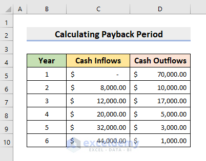
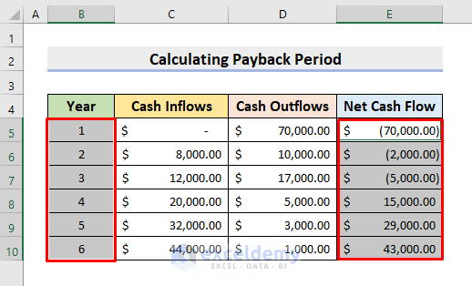
Input data. In this example, we’ll type Cash Inflows and Cash Outflows of 6 years. See the picture below.

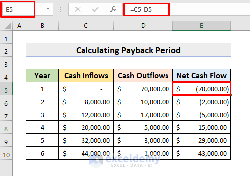
Calculate the net/cumulative cash flow. Select cell E5.
Type the formula:

=C5-D5

Press Enter.
Use AutoFill to complete the rest.

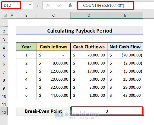
Step 2 – Determining Break-Even Point

The point of no profit and no loss is the break-even point. We obtain the break-even point of a project when the net cash flows exceed the initial investment.

Select cell D12.
Insert the formula:

=COUNTIF(E5:E10,"<0")

The COUNTIF function counts the number of years where the net cash flow is negative.

Press Enter to get the break-even point.

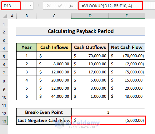
Step 3: Obtaining Last Negative Cash Flow

If our dataset is large, we won’t be able to find the last negative cash flow manually.

Click on cell D13.
Input the formula:

=VLOOKUP(D12, B5:E10, 4)

Press Enter.

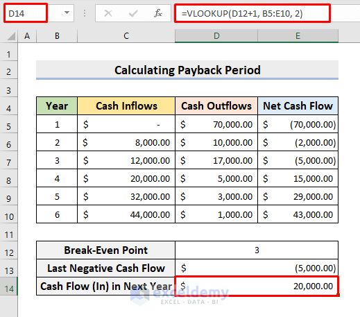
Step 4 – Using VLOOKUP to Find Next Year’s Cash Flow

Choose cell D14.
Type the formula:

=VLOOKUP(D12+1, B5:E10, 2)

Press Enter to return the result.

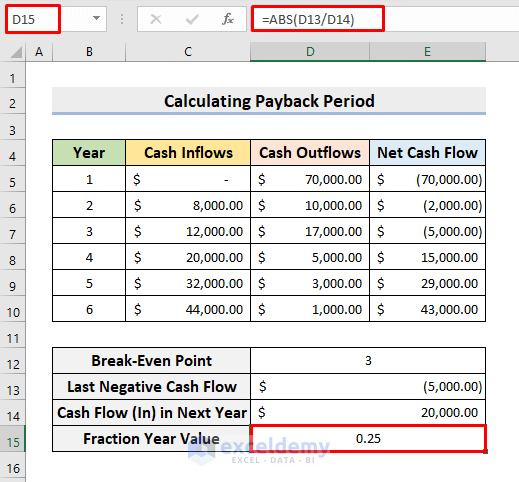
Step 5 – Computing Fractional Year Value with ABS Function

Select cell D15.
Insert the formula:

=ABS(D13/D14)

Press Enter.

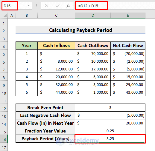
Step 6 – Calculating Payback Period

Click cell D16.
Type the formula:

=D12 + D15

Press Enter.
You’ll get the accurate payback period in years.

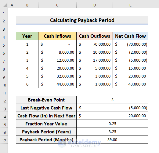
To convert it to months, in cell D17, input the formula:

=D16*12

Press Enter to get the output in months format.

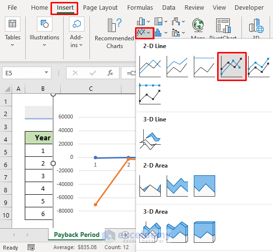
Step 7 – Inserting Chart to Show Payback Period in Excel

Choose the ranges B5:B10 and E5:E10 (hold Ctrl while selecting).

Go to Insert, select Line Chart, and choose 2-D Line Chart with Markers.

In that chart, you’ll see the approximate value where the series crosses the X-axis which is the payback period.
But with this chart, we can’t get the exact value as we have shown earlier.

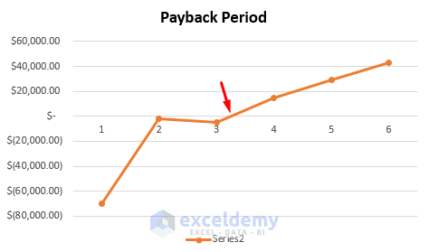
Here’s how final output is displayed.

Download Practice Workbook

Download the following template to practice by yourself.

Calculate Payback Period.xlsx

<< Go Back to Excel Cash Flow Formula | Excel Formulas for Finance | Excel for Finance | Learn Excel

Get FREE Advanced Excel Exercises with Solutions!

3 thoughts on “How to Calculate Payback Period in Excel (With Easy Steps)”

Aline says:

Nov 18, 2022 at 11:04 PM

Hello, the computation of the fraction year value doesn’t work if the first positive CF has a smaller absolute value than the last negative CF. How do I adjust the formula?

Nafez says:

Sep 29, 2023 at 1:08 PM

Hello I would like to thank you for your effort, and invet you to visit Qatar

1. Shamima Sultana says:
  
  Oct 1, 2023 at 3:50 PM
  
  Hello Nafez,
  
  You are most welcome and thanks for you invitation to visit Qatar.
  
  Regards
  ExcelDemy