In this article, we will demonstrate 3 methods to calculate Discounted Payback Period in Excel.
What Is Discounted Payback Period?
Discounted payback period refers to the time taken (in years) by a project to recover the initial investment based on the present value of the future cash flows generated by the project. It is an essential metric when evaluating the profitability and feasibility of any project.
How to Calculate Discounted Payback Period in Excel: 3 Ways
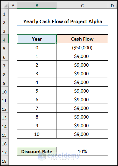
Consider the Yearly Cash Flow of Project Alpha dataset in cells B4:C15. In this dataset, we have the Years from 0 to 10 and their Cash Flows respectively. An initial investment of $50,000 is made at the start of the project and a positive cash flow of $9,000 is recorded at the end of each year. In addition, we’ve chosen a Discount Rate of 10% for this project. Let’s calculate the Discounted Payback Period.
We used Microsoft Excel 365 version, but you may use any other version at your disposal.
Method 1 – Using PV Function
The most obvious way to calculate the discounted payback period in Excel is using the PV function to calculate the present value, then obtaining the payback period of the project.
Steps:
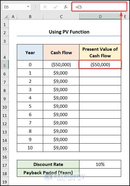
- In cell D5, enter the following formula:
=C5
Cell C5 refers to the Cash Flow at Year 0.
- In cell D6, enter the following formula:
=-PV($D$17,B6,0,C6,0)
In this formula, cell D17 is the Discount Rate while cells B6 and C6 are Year 1 and Cash Flow of $9,000 respectively. The Present Value of Cash Flow is negative, so we use a negative sign to make the value positive.
Note: Always use Absolute Cell Reference by pressing the F4 key on your keyboard.
Formula Breakdown:
- -PV($D$17,B6,0,C6,0) → returns the present value of an investment, that is the total amount a series of future payments is worth now. $D$17 is the rate argument that refers to the Discount Rate. B6 represents the nper argument, which is the annual number of payments. 0 is the pmt argument which indicates the payment amount made each period. C6 points to the optional fv argument, which is the future value of the cash flow. 0 represents the optional type argument, which refers to the payment made at the end of the year.
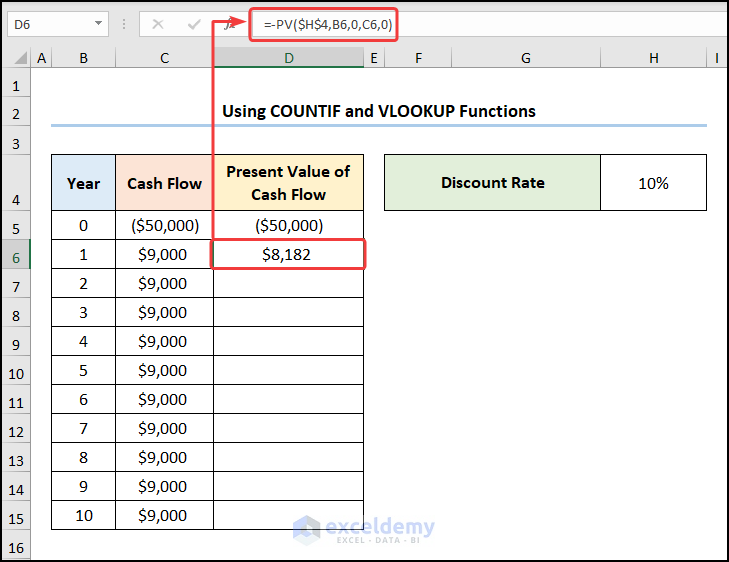
- Output → $8,182

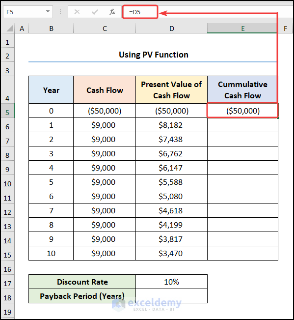
- In cell E5, enter the formula below:
=D5
Cell D5 represents the Present Value of Cash Flow.
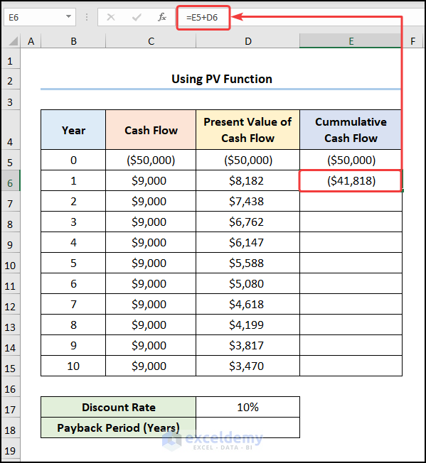
- In cell E6, enter the formula below:
=E5+D6
Cell E5 is the Cumulative Cash Flow while cell D6 is the Present Value of Cash Flow.
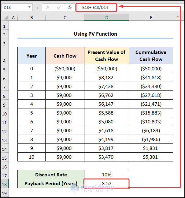
- Calculate the payback period by using the formula below:
=B13+-E13/D14
Cell B13 is Year 8 while cells E13 and D14 indicate values of $1,986 and $3,817 respectively.
Read More: How to Calculate Payback Period in Excel
Method 2 – Using IF Function
Steps:
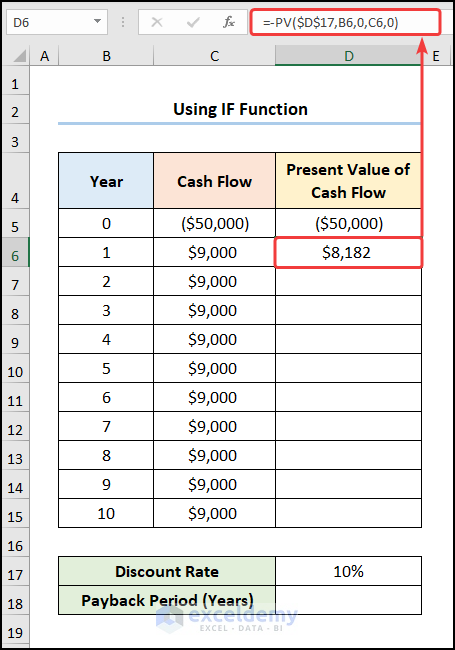
- In cell D6, enter the formula below:
=-PV($D$17,B6,0,C6,0)
Cell D17 is the Discount Rate while cells B6 and C6 are Year 1 and Cash Flow of $9,000 respectively.
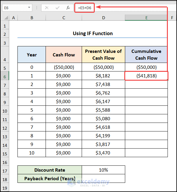
- In cell E6, enter the formula below:
=E5+D6
Cell E5 is the Cumulative Cash Flow while cell D6 is the Present Value of Cash Flow.
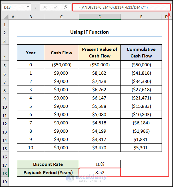
- Calculate the Payback Period (Years) by using the formula below:
=IF(AND(E13<0,E14>0),B13+(-E13/D14),"")
Formula Breakdown:
- IF(AND(E13<0,E14>0),B13+(-E13/D14),””) → becomes
- IF(TRUE,B13+(-E13/D14),””) → the IF function checks whether a condition is met and returns one value if TRUE and another value if FALSE. Here, the IF function returns the value of B13+(-E13/D14) which is the value_if_true argument. Otherwise, it would return “” (BLANK) which is the value_if_false argument.
- Output → 8.52
Method 3 – Using VLOOKUP and COUNTIF Functions
We can also employ the COUNTIF and VLOOKUP functions to calculate the discounted payback period.
Steps:
- In cell D6, enter the formula below:
=-PV($H$4,B6,0,C6,0)
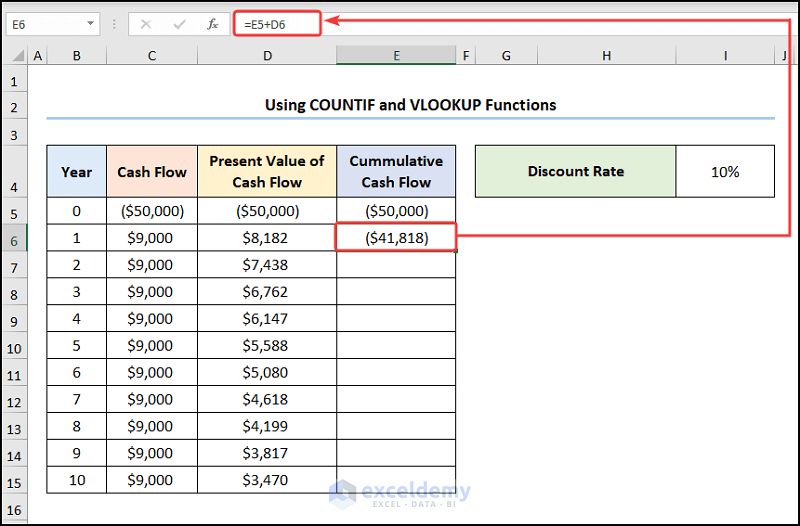
- In cell E6, enter the formula below:
=E5+D6
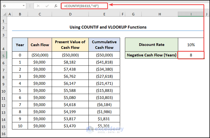
- In cell I5, use the COUNTIF function as follows:
=COUNTIF(E6:E15,"<0")
Formula Breakdown:
- COUNTIF(E6:E15,”<0″) → counts the number of cells within a range that meet the given condition. Here, E6:E15 is the range argument that refers to the Cumulative Cash Flow. “<0” represents the criteria argument that returns the count of the years with negative cash flow values.
- Output → 8
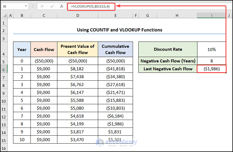
- In cell I6 use the VLOOKUP function as follows to determine the Last Negative Cash Flow:
=VLOOKUP(I5,B5:E15,4)
Cell I5 is the Negative Cash Flow (Years) value of 8.
Formula Breakdown:
- VLOOKUP(I5,B5:E15,4) → looks for a value in the left-most column of a table and returns a value in the same row from a specified column. Here, I5 (the lookup_value argument) is mapped from the B5:E15 (table_array argument) array. 4 (col_index_num argument) represents the column number of the lookup value.
- Output → ($1,986)
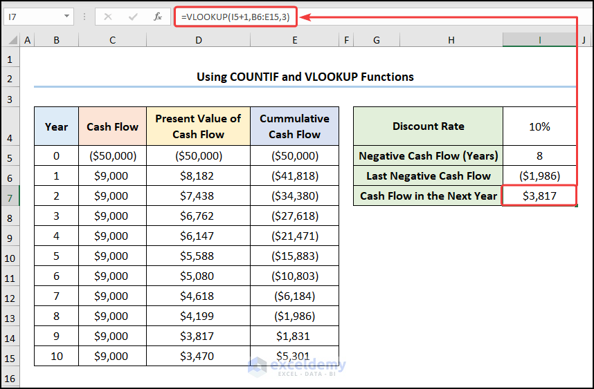
- Similarly, determine the Present Value of Cash Flow for the next year as follows:
=VLOOKUP(I5+1,B6:E15,3)
Formula Breakdown:
- VLOOKUP(I5+1,B6:E15,3) → I5+1 (the lookup_value argument) is mapped from the B6:E15 (table_array argument) array. 3 (col_index_num argument) represents the column number of the lookup value.
- Output → $3,817
- Calculate the Fraction Period (Years) using the ABS function as follows:
=ABS(I6/I7)
Cells I6 and I7 represent the Last Negative Cash Flow and the positive Cash Flow in the Next Year.

- Calculate the Payback Period (Years) by adding the values of cells I5 and I8.
=I5+I8
Cell I5 is the Negative Cash Flow (Years) while cell I8 is the Fraction Period (Years).
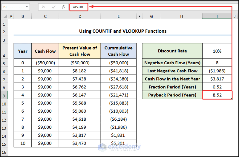
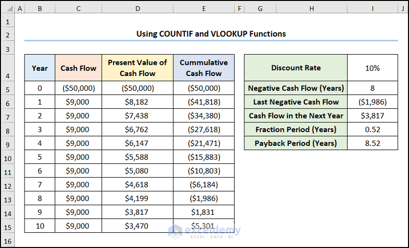
The result should look like the screenshot below.
Read More: Calculating Payback Period in Excel with Uneven Cash Flows
What Is Uneven Cash Flow?
Uneven Cash Flow refers to a series of unequal payments made over a certain period, for instance a series of $5000, $8500, and $10000 made over 3 years. So the primary difference between even and uneven cash flows is that in even cash flows the payment values remain equal over a given period, whereas the payment values can be different in uneven cash flows.
Calculating Discounted Payback Period for Uneven Cash Flow
So far, we’ve only considered cases of even cash flows. Now let’s calculate the discounted payback period for uneven cash flow.
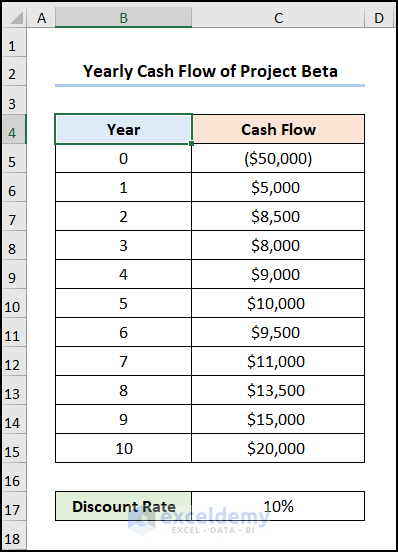
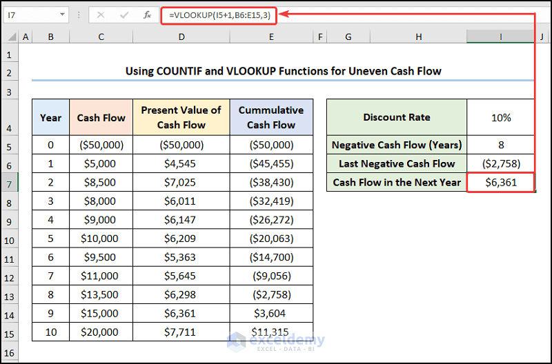
Consider the Yearly Cash Flow of Project Beta dataset shown in the B4:C15 cells below. We have the Years from 0 to 10 and their uneven Cash Flows respectively. As in the previous example, we’ve also set a Discount Rate of 10% for this project.
Steps:
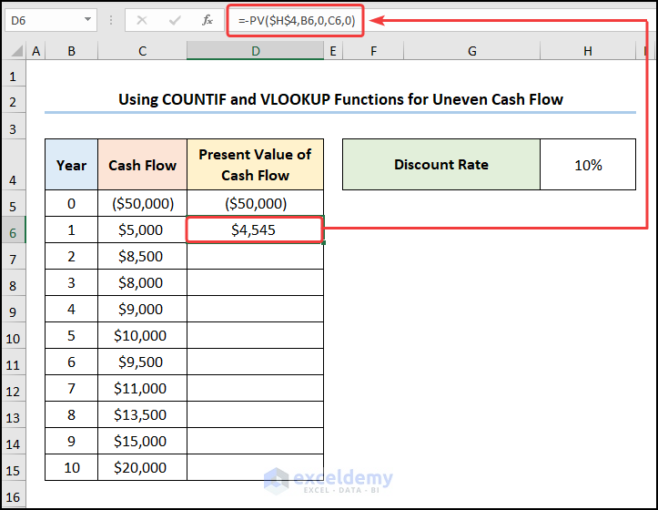
- In cell D6, enter the formula below:
=-PV($H$4,B6,0,C6,0)
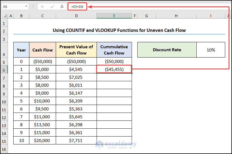
- In cell E6, enter the formula below:
=E5+D6
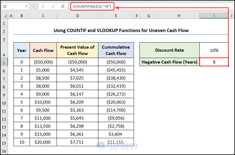
- In cell I5, compute the Negative Cash Flow (Years) as follows:
=COUNTIF(E6:E15,"<0")
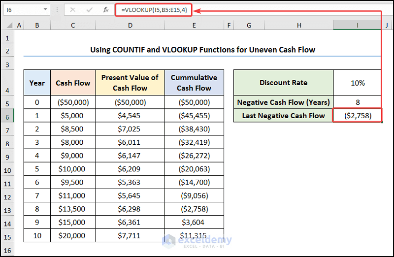
- In cell I6, calculate the Last Negative Cash Flow value with the formula below:
=VLOOKUP(I5,B5:E15,4)
- Determine the Present Value of Cash Flow for the next year with this formula:
=VLOOKUP(I5+1,B6:E15,3)
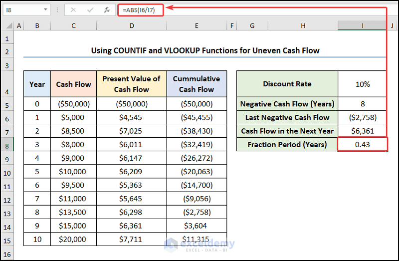
- Calculate the Fraction Period (Years) using the ABS function as follows:
=ABS(I6/I7)
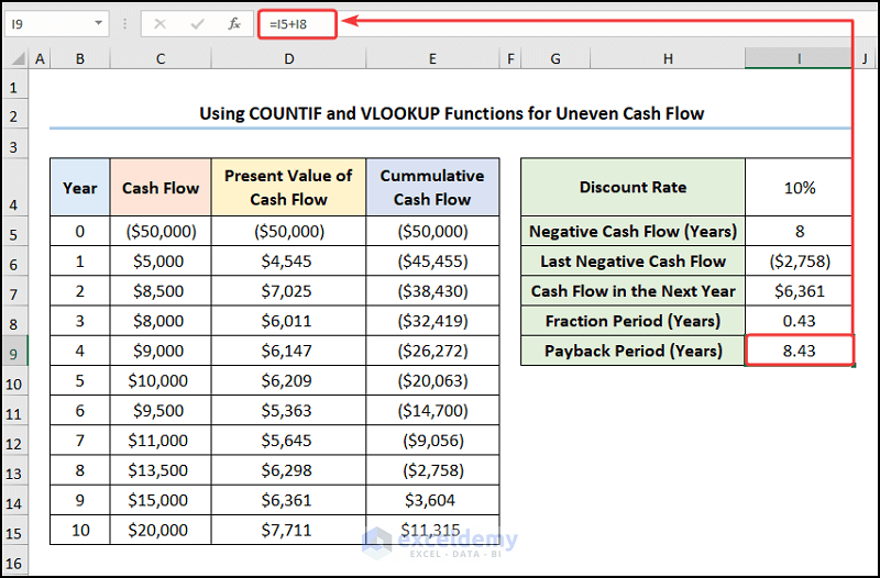
- Add the values of cells I5 and I8 to obtain the Payback Period (Years):
=I5+I8
For sake of brevity, we have skipped some of the other relevant examples of Uneven Cash Flow.
Read More: How to Apply Discounted Cash Flow Formula in Excel
Download Practice Workbook
Related Articles
- How to Calculate Operating Cash Flow in Excel
- How to Calculate Incremental Cash Flow in Excel
- How to Create a Cash Flow Waterfall Chart in Excel
<< Go Back to Excel Cash Flow Formula | Excel Formulas for Finance | Excel for Finance | Learn Excel
Get FREE Advanced Excel Exercises with Solutions!
