How to Calculate the Discounted Cash Flow in Excel – 3 Easy Steps

What Is the Discounted Cash Flow?

What your future cash flow is worth in terms of today’s value is known as Discounted Cash Flow.

Formula to Calculate The Discounted Cash Flow

The total amount of the cash flow for every period of time divided by one increment of the discount rate raised to the power of the period count is the Discounted Cash Flow (DCF) formula.

CFt = Cash flow in period t (time)
r = Discount rate
t = Period of time (1,2,3,……,n)

Step 1– Calculatiing the Present Value

Steps:

• Consider a cash flow for every year. Here, $50,000.

• Consider the Discount Rate. It symbolizes the interest rate to calculate the future cash flow based on the current situation. Here, 10% as the discount rate.
• Enter the following formula to calculate the present value after 1 year.

C6 = Cash Flow after the first year
G5 = Discount Rate
B6 = Period of Time

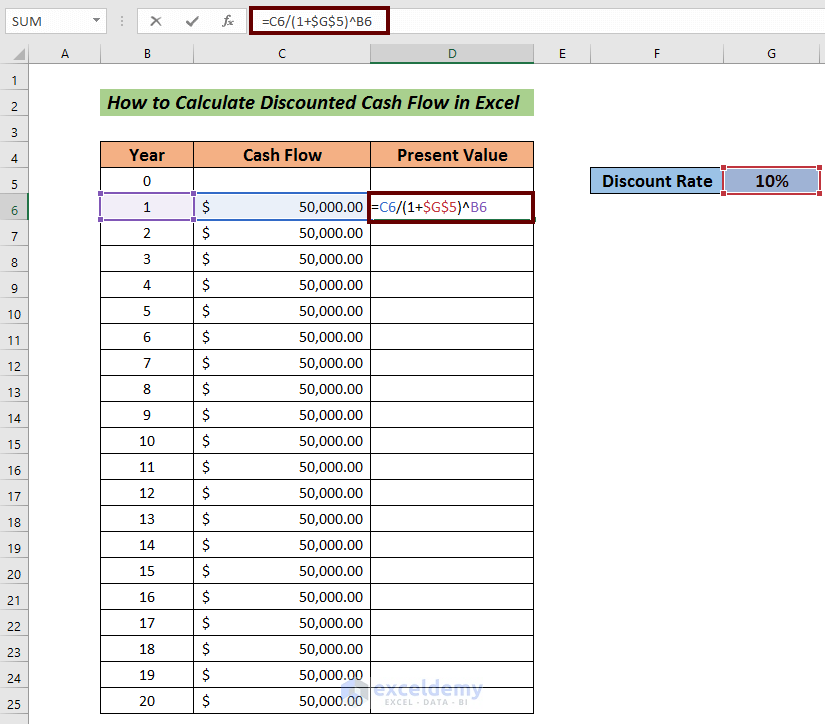
• Press ENTER to see the output.

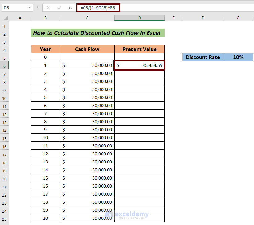
• Drag down the Fill Handle to AutoFill the rest of the cells.

Read More: How to Calculate Annual Cash Flow in Excel

Step 2 – Calculating the Discounted Cash Flow in Excel

Steps:

• Estimate the total value of the Present Value. Enter the following formula:

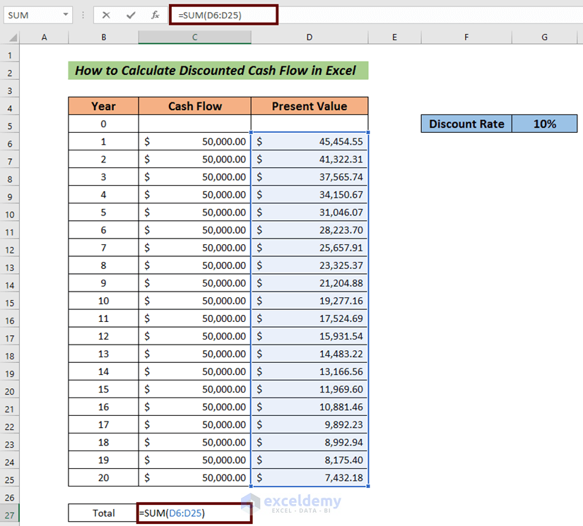
• Press ENTER to see the result.

The total present value of the payment is $425,678.19. The total cash flow is $1,000,000.

Read More: How to Calculate Incremental Cash Flow in Excel

Step 3 – Validation of the Discounted Cash Flow Calculation in Excel

Steps:

• Calculate the profit of the investments in a column. Here, a profit of 10% was assumed based on the invested amount and listed in the Return column.
• Use the following formula to calculate the return:

F6 = End Value of the previous year
I5 = Return Rate

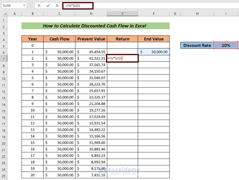
• Press ENTER to see the return value.

• Calculate the End Value using the following formula:

F6 = End Value of the previous year
C7 = Cash Flow of the current year
E7 = Return value of that year

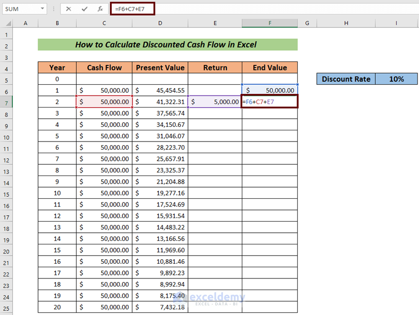
• Press ENTER to see the output.

• AutoFill the Return and End Value columns.

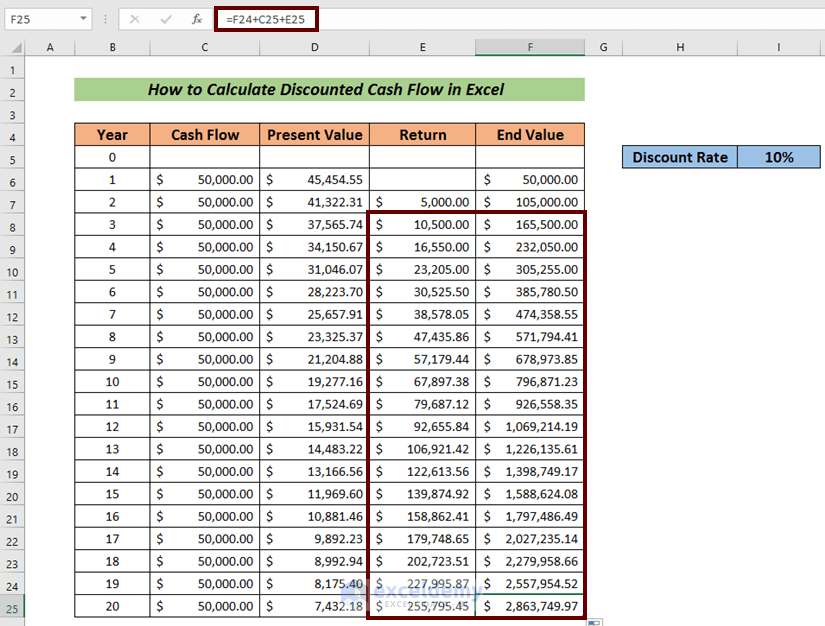
The projected End Value after 20 years is calculated.

• Consider the total present value as the Lump Sum value for the beginning of the investment.
• Enter the following formula to get the Lump Sum value for the following year:

G5 = Lump Sum Value
J5 = Discount rate

• Press ENTER to see the Lump Sum value.

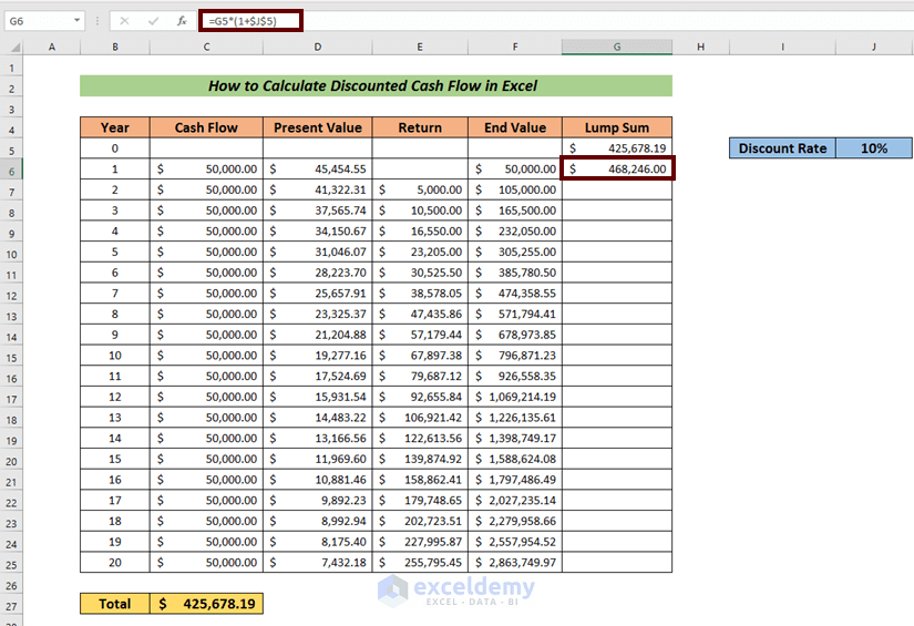
• AutoFill the rest of the cells.

The End Value and the Lump Sum value is equal at the end of the time period. The Discounted Cash Flow calculation is accurate.

Read More: How to Forecast Cash Flow in Excel

Download Practice Workbook

Related Articles

• How to Calculate Free Cash Flow in Excel
• How to Calculate Cumulative Cash Flow in Excel
• How to Draw a Cash Flow Diagram in Excel
• How to Track Cash Flow in Excel
• How to Create a Personal Cash Flow Statement in Excel
• How to Calculate Operating Cash Flow Using Formula in Excel
• How to Calculate Payback Period in Excel
• How to Calculate Payback Period with Uneven Cash Flows
• How to Apply Discounted Cash Flow Formula in Excel
• How to Calculate Operating Cash Flow in Excel

<< Go Back to Excel Cash Flow Formula | Excel Formulas for Finance | Excel for Finance | Learn Excel