This is the template:
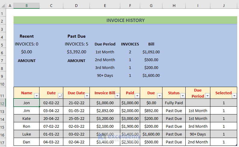
Example 1 – Keeping Track of Invoices and Payments in Excel by Showing Recent and Past Invoice Amounts
Steps:
- Create a chart like the following:
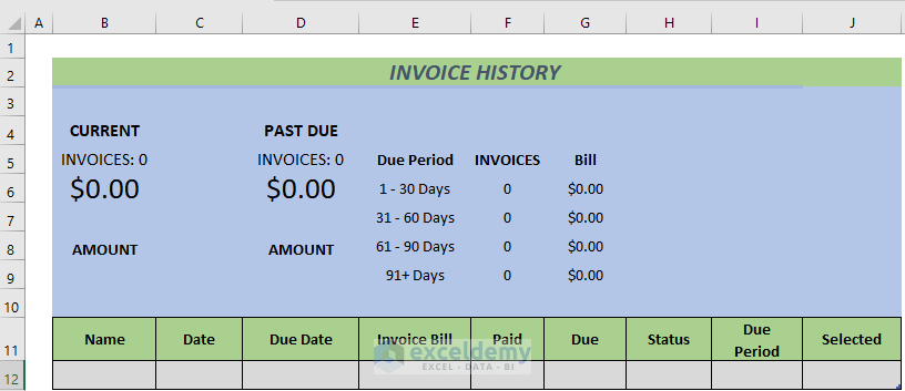
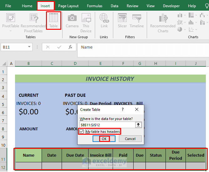
- Select B11:J12 and go to Insert >> Table
- Check My table has headers.
- Click OK.
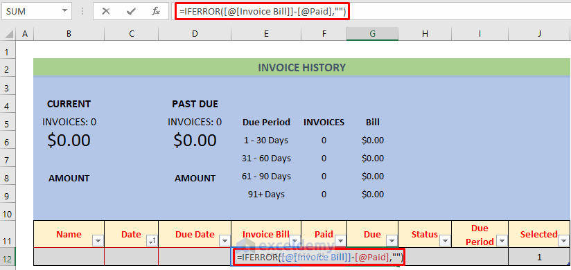
- Enter this formula in G12 and press ENTER.
=IFERROR([@[Invoice Bill]]-[@Paid],"")It calculates dues or outstanding amounts.
- Use this formula in H12 and press ENTER.
=IFERROR(IF(OR([@[Invoice Bill]]="",[@Date]="",[@[Due Date]]="", [@[Due Date]]<[@Date]),"Error",IF([@Due]=0,"Fully Paid", IF([@Due]>0,IF(PD<[Due Date],"Recent",IF(PD=[@[Due Date]], "Due Today",IF(PD>[@[Due Date]],"Past Due"))),IF([@Due]<0, "Get Return")))),"")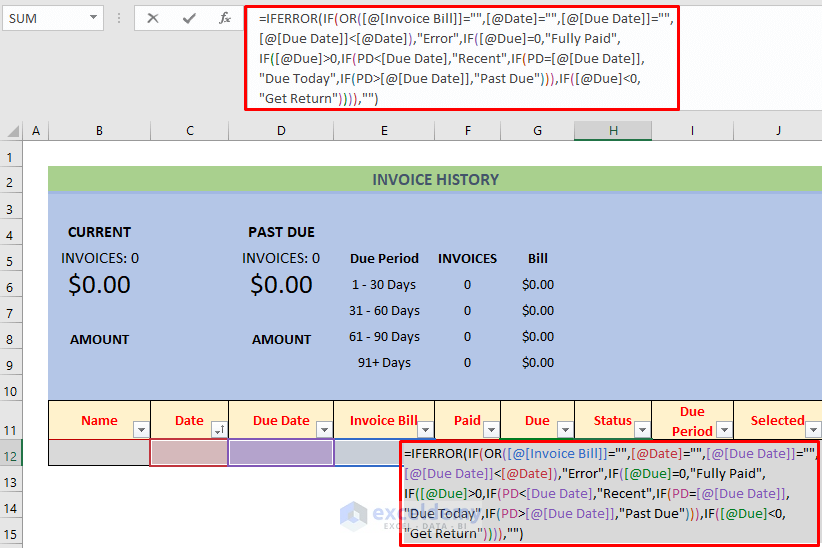
It shows paid invoice and status of the due. PD is the named range for the present date. It also informs of possible returns to client. the IF Function was used.
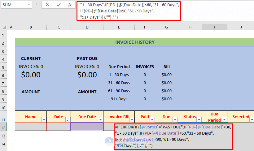
- Use this formula in I12 and press ENTER.
=IFERROR(IF([@Status]="Past Due",IF(PD-[@[Due Date]]<30, "1st Month",IF(PD-[@[Due Date]]<60,"2nd Month", IF(PD-[@[Due Date]]<90,"3rd Month", "90+ Days"))),""),"")It returns the duration of the due.
.
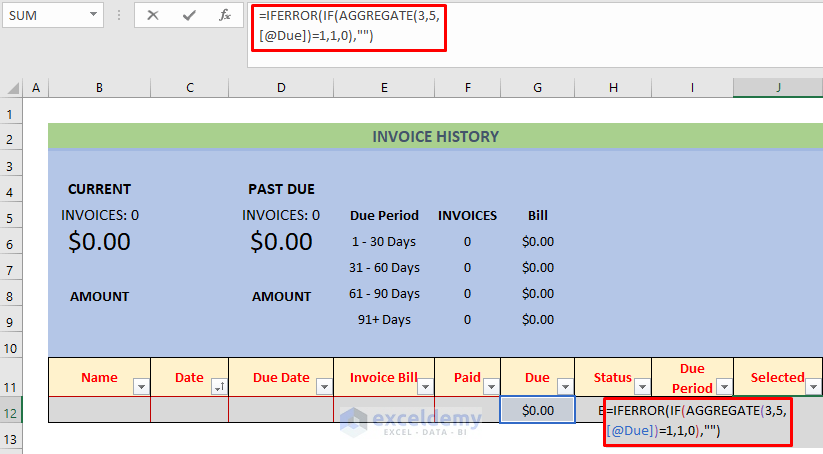
- Enter the following formula in J12 and press ENTER.
=IFERROR(IF(AGGREGATE(3,5, [@Due])=1,1,0),"")The formula returns information on invoice data. It uses the AGGREGATE Function.
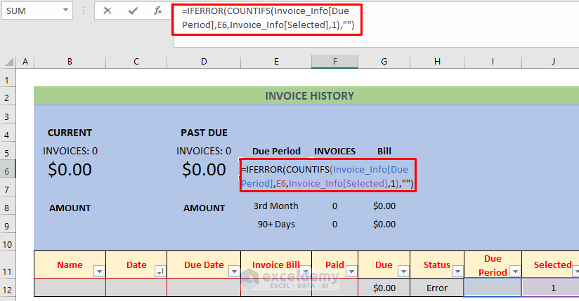
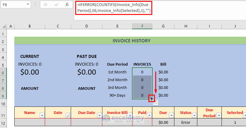
- Copy the formula below to F6 and press ENTER.
=IFERROR(COUNTIFS(Invoice_Info[Due Period],E6,Invoice_Info[Selected],1),"")It returns the number of invoices in a period of time.
- Press ENTER and use the Fill Handle to AutoFill cells up to F9.
- Enter the following formula in G6, press ENTER and use the Fill Handle to AutoFill cells up to G9.
=IFERROR(SUMIFS(Invoice_Info[Due],Invoice_Info[Due Period],E6,Invoice_Info[Selected],1),"")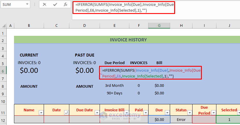
It stores invoices within a given period.
- Use this formula to store recent invoices in B5:
=IFERROR("INVOICES: "&COUNTIFS(Invoice_Info[Status],"Recent",Invoice_Info[Selected],1)+COUNTIFS(Invoice_Info[Status],"Due Today",Invoice_Info[Selected],1),"")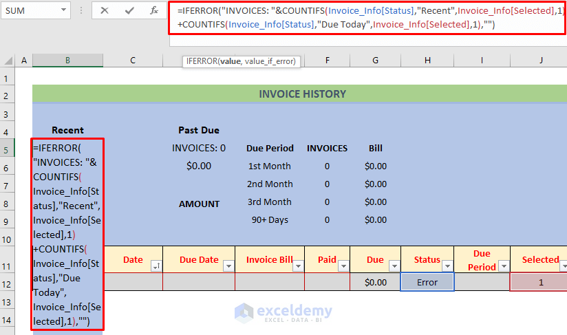
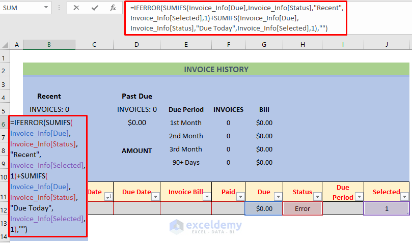
- Use the formula in B6.
=IFERROR(SUMIFS(Invoice_Info[Due],Invoice_Info[Status],"Recent", Invoice_Info[Selected],1)+SUMIFS(Invoice_Info[Due], Invoice_Info[Status],"Due Today",Invoice_Info[Selected],1),"")It returns total invoices in recent times in B6.
- Enter the following formula in D5 and press ENTER.
=IFERROR("INVOICES: "&COUNTIFS(Invoice_Info[Status], "Past Due",Invoice_Info[Selected],1),"")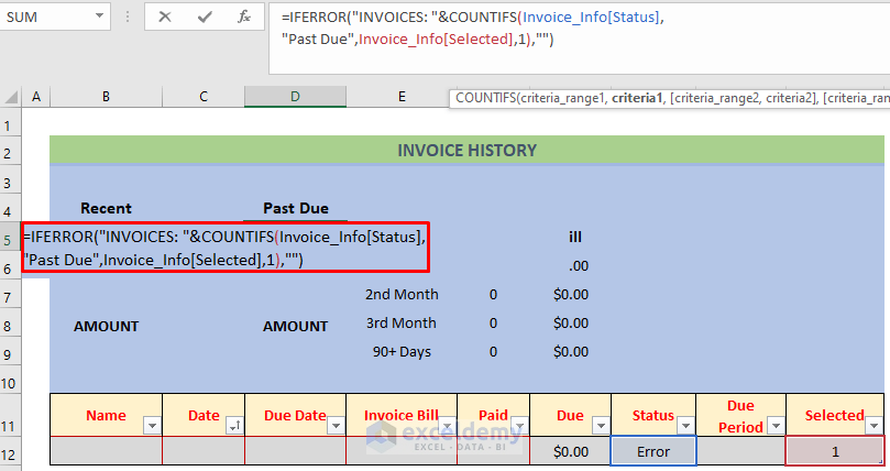
It calculates the number of past dues in D5.
- Enter the following formula in D6 and press ENTER.
=IFERROR(SUMIFS(Invoice_Info[Due],Invoice_Info[Status], "Past Due",Invoice_Info[Selected],1),"")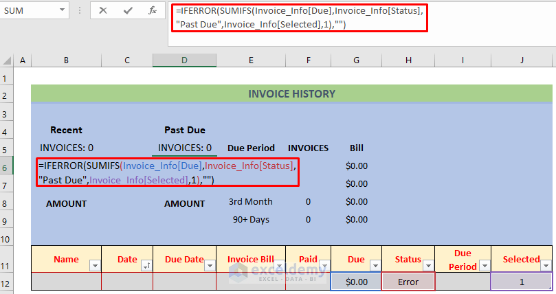
It stores past dues in D5.
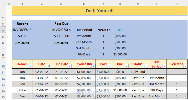
- The following chart is an example of an invoice tracker with random data:
New entries will update the invoice history.
Read More: How to Keep Track of Customer Orders in Excel
Example 2 – Using the Table Feature to Keep Track of Invoices and Payments in Excel
Steps:
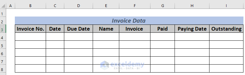
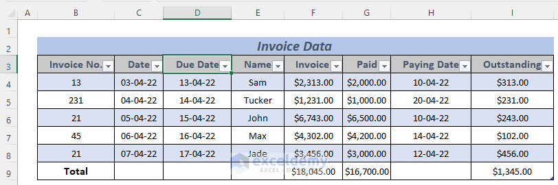
- Create a table like the following:
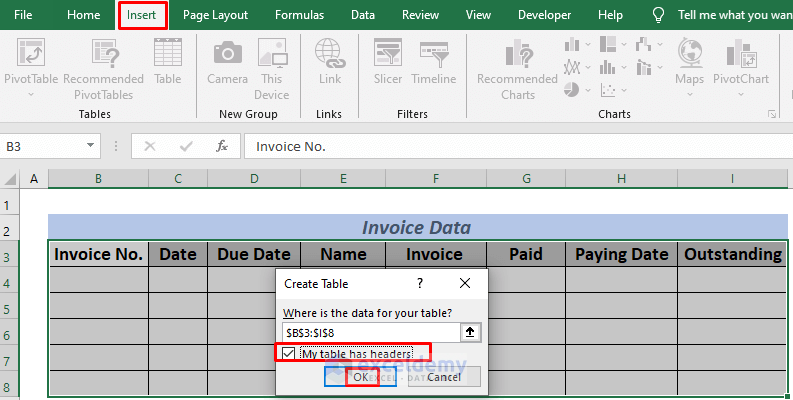
- Select B3:I8 and go to Insert >> Table
- Check My table has headers and click OK.
- Enter the following formula in F9.
=SUM(F4:F8)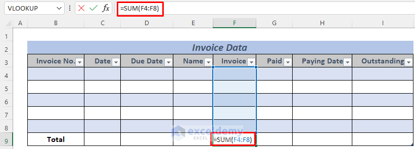
It stores the total invoice using the SUM function.
- Use the following formula in G9.
=SUM(G4:G8)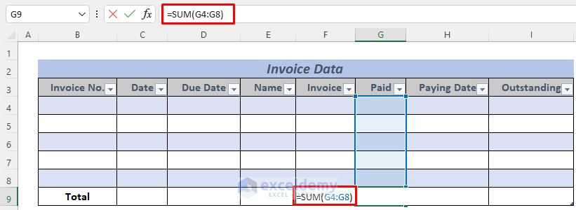
It stores the total paid amount.
- Add the formula below.
=SUM(I4:I8)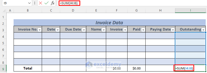
It stores the total outstanding.
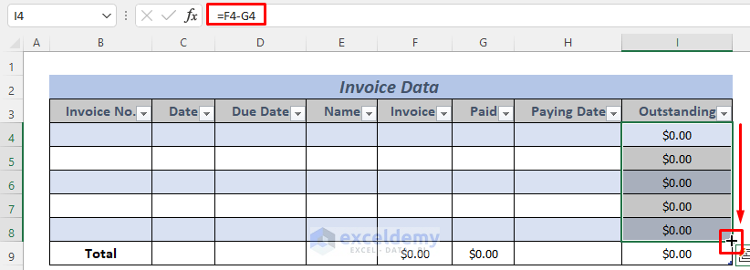
- Use the formula below in I4.
=F4-G4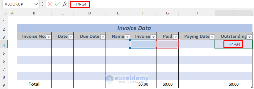
It calculates row-wise outstanding.
- Use the Fill Handle to AutoFill cells up to I8.
The following chart showcases a template with random data to keep track of invoices and payments in Excel:
Read More: How to Keep Track of Customer Payments in Excel
Example 3 – Storing Customer Information Automatically to Keep Track of Invoices and Payments in Excel
Steps:
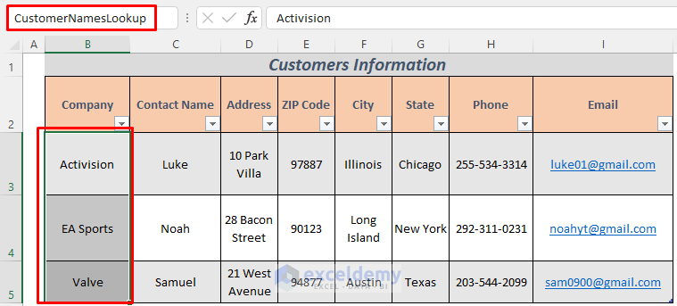
- Store your customers’ information in a new sheet.
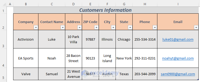
- Create a table like the one in the following picture in another sheet.
- To make an invoice tracker for today, use the TODAY Function for the date.
=TODAY()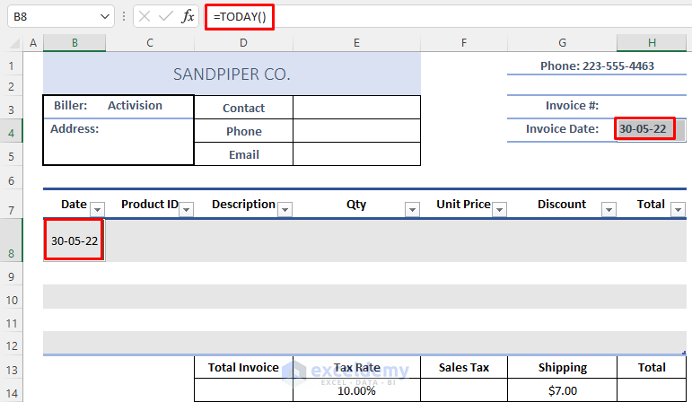
- Create a named range for the billing company. Here, CustomerNamesLookup.
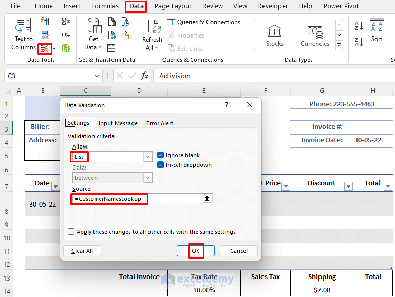
- A data validation list for the billing company was created. Select C3 and go to Data >> Data Validation
- Select List in Allow: and set the Source as ‘=CustomerNamesLookup’.
- Click OK.
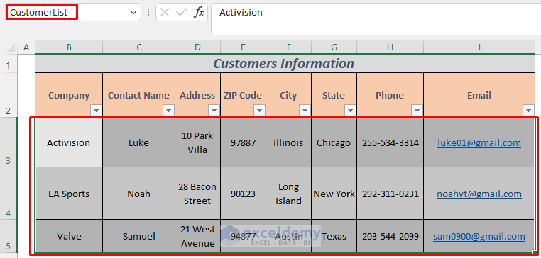
- Create another name for the range B3:I5. CustomerList,here.
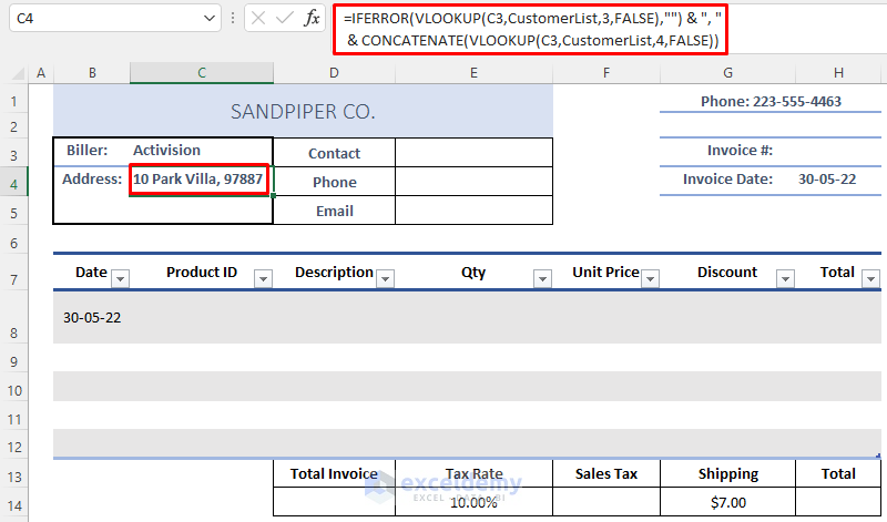
- Enter the following formula in C4.
=IFERROR(VLOOKUP(C3,CustomerList,3,FALSE),"") & ", " & CONCATENATE(VLOOKUP(C3,CustomerList,4,FALSE))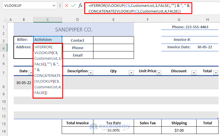
It stores the address of the billing company. The VLOOKUP function looks for the CustomerList and the CONCATENATE Function for address and ZIP Code.
- Press ENTER and you will see your customer’s address.
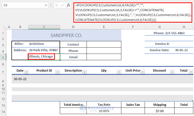
- Enter the following formula in C5:
=IF(VLOOKUP(C3,CustomerList,4,FALSE)="","",IF(VLOOKUP(C3,CustomerList,5,FALSE)<>"",CONCATENATE(VLOOKUP(C3,CustomerList,5,FALSE),", ",VLOOKUP(C3,CustomerList,6,FALSE)),CONCATENATE(VLOOKUP(C3,CustomerList,6,FALSE))))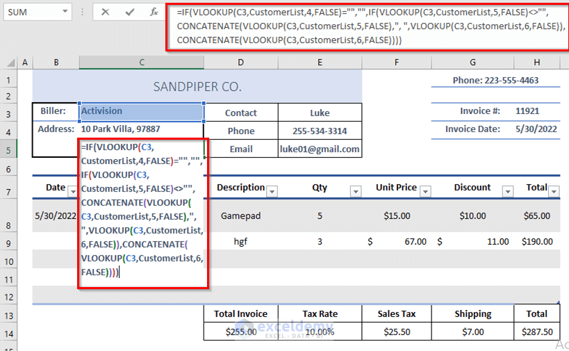
- Press ENTER
It returns the name of the city and state.
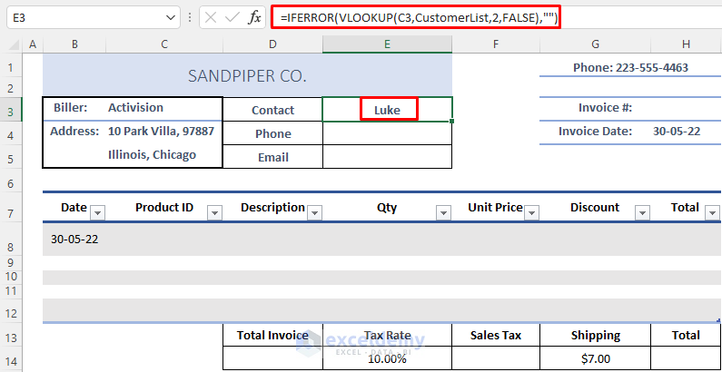
- Enter the formula below in E3.
=IFERROR(VLOOKUP(C3,CustomerList,2,FALSE),"")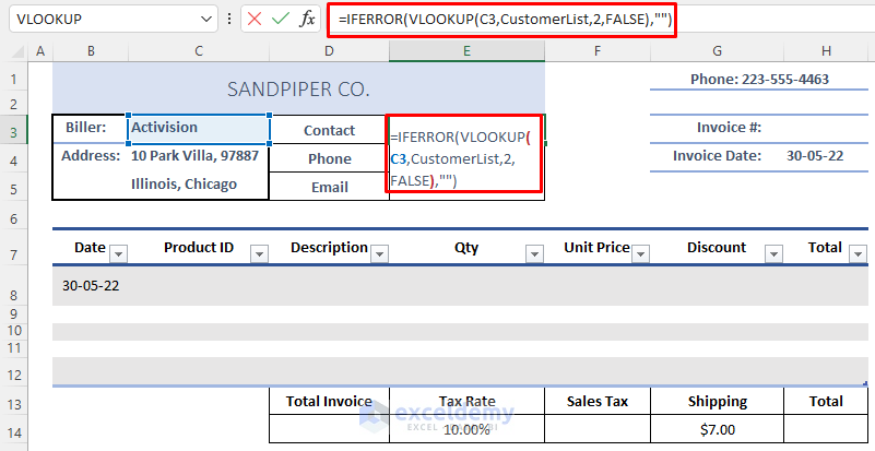
- Press ENTER
It returns the contact person’s name.
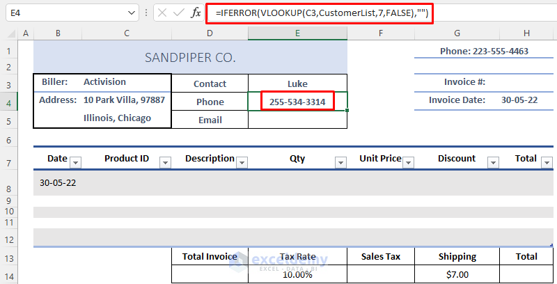
- Use the following formula in E4:
=IFERROR(VLOOKUP(C3,CustomerList,7,FALSE),"")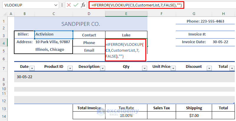
- Press ENTER.
It returns the phone number.
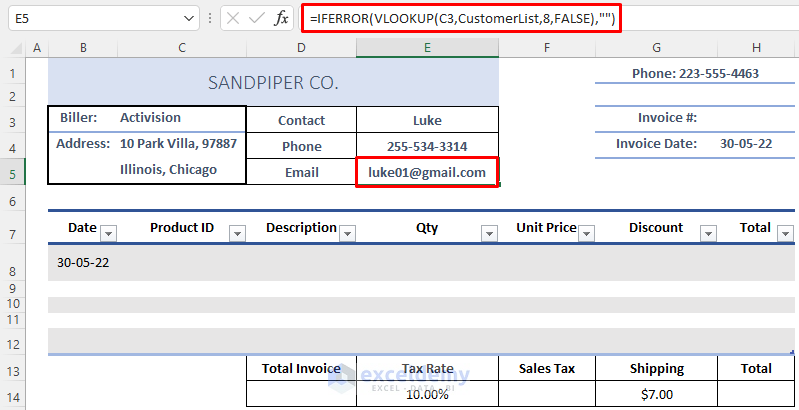
- Enter the following formula in E5:
=IFERROR(VLOOKUP(C3,CustomerList,8,FALSE),"")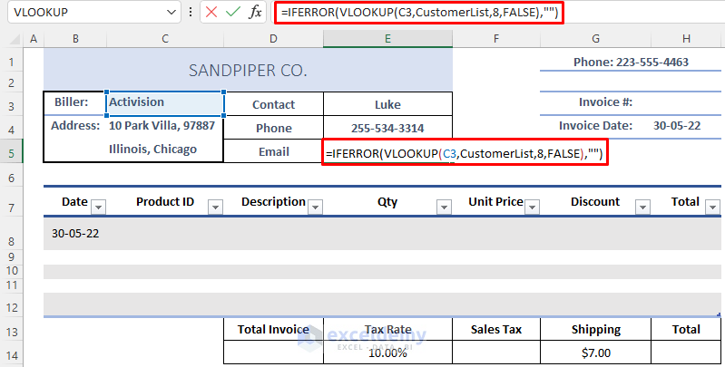
- Press ENTER.
It returns the customer’s email ID.
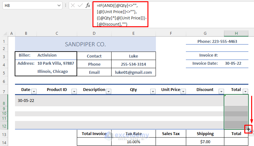
- Use the formula below in H8.
=IF(AND([@Qty]<>"",[@[Unit Price]]<>""),([@Qty]*[@[Unit Price]])-[@Discount],"")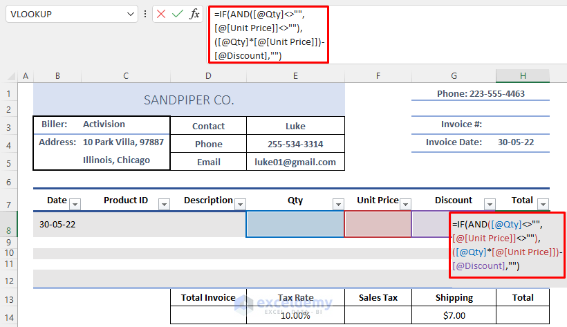
- Press ENTER and AutoFill cells up to H12.
It returns the total invoice for your product.
- Choose a name for range B8:H12. Here, InvoiceTable.
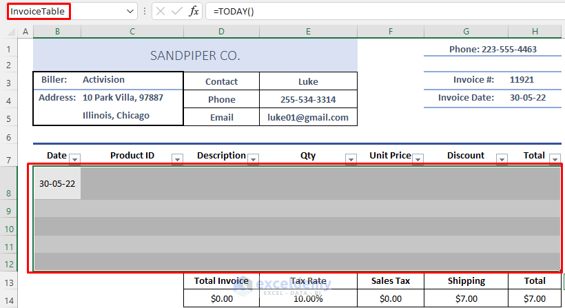
- Enter the formula below and press ENTER.
=SUM(InvoiceTable[Total])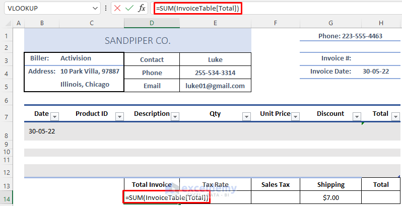
It stores the total amount of the invoice.
- To determine the tax amount, enter the following formula in F14 and press ENTER.
=D14*E14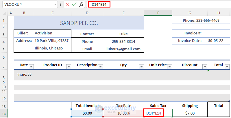
- Use the formula below in H14 and press ENTER.
=D14+F14+G14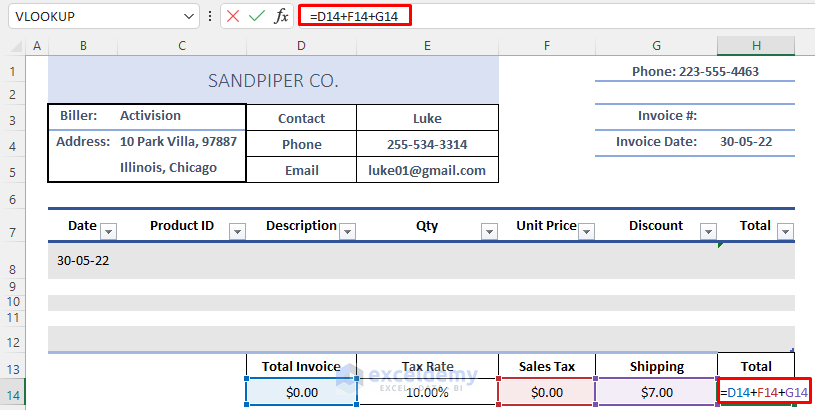
It returns the amount to be paid.
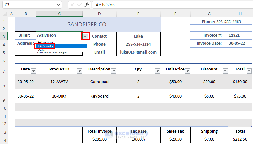
The following chart showcases a template with random data:
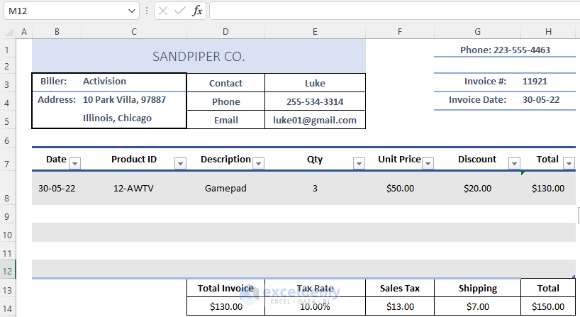
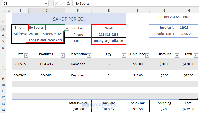
Suppose EA Sports wants to order the following items. Insert the products and invoice information and select EA Sports from the drop down list to find their contact information.
- After choosing EA Sports from the data validation list, you can easily contact them.
Practice Section
Use the following template to practice:
Download Invoice & Payment Template (Free)
Related Articles
- How to Keep Track of Clients in Excel
- How to Make a Sales Tracker in Excel
- How to Create a Task Tracker in Excel
- How to Create a Daily Task Sheet in Excel
- How to Create a Progress Tracker in Excel
- How to Create Real Time Tracker in Excel
<< Go Back to Create a Tracker in Excel | Tracker in Excel | Excel Templates
Get FREE Advanced Excel Exercises with Solutions!

Hello,
I hope all is well!
I am trying to mirror your steps, and I’m having an issue when I get to the G6 Step.
I keep writing the following formula =IFERROR(COUNTIFS(Invoice_Info[Due Period],E6,Invoice_Info[Selected],1),””)but every time i press enter it gives me an error. However, i’m not sure what the Invoice_Info is. This is what i end up doing – =IFERROR(SUMIFS(Table1[Due],Table1[Due Period],E6,Table1[Selected],1),””) but i’m not if that correct either.
Hi! Thanks for asking. As the article was to provide some templates, I didn’t go in detail with the formula. Here, Invoice_Info is a named range. It refers to the range B12:J17 of the ‘template 1’ sheet. To create a named range, you need to select your desired range of cells, then go to Data Tab >> Define Name and after that, give a name of that range. The advantage is that, you can use that range by inserting it’s name anywhere in the worksheet or workbook. You don’t have to select the range every time you use it in a formula. Hope this solves your problem.