Step 1 – Make Dataset for Contact Details
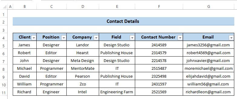
The contact details include specific information about that client, such as their contact number, email address, company name, related field, and position.
- Make a new sheet.
- Put some client details in your worksheet.
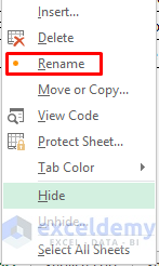
- To change the sheet name, right-click on the sheet name. A Context Menu will pop up.
- Click on Rename.

- We set our worksheet name as ‘Contact Details’.
- Press Enter.
Read More: How to Keep Track of Customer Orders in Excel
Step 2 – Create Client Service Details
- Press + in the toolbar with the sheet names to create a new sheet.
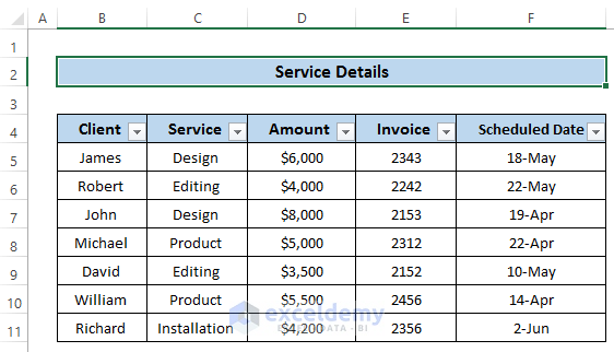
- Put information that includes the service name, the amount of money that cost on the particular service, and the scheduled date to give the service.
- Right-click on the sheet name.
- Click on Rename.
- Change the worksheet to ‘Service Details’.
Read More: How to Keep Track of Customer Payments in Excel
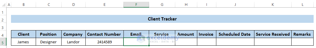
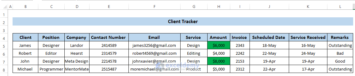
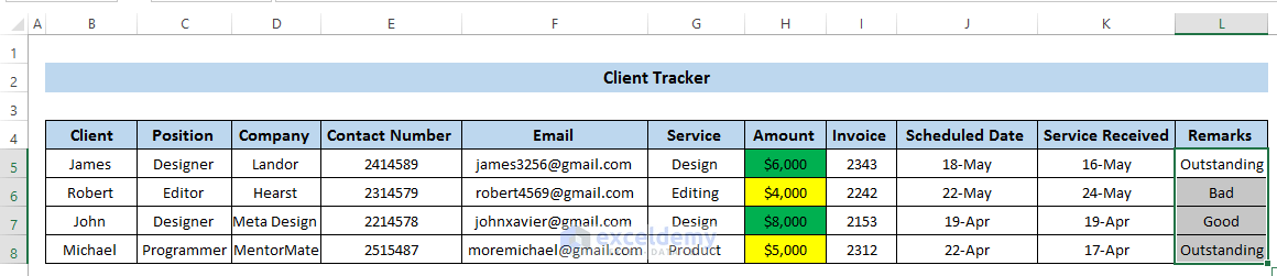
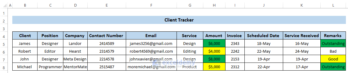
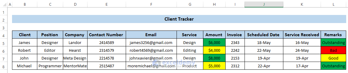
Step 3 – Generate Client Tracker
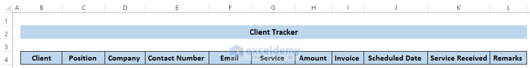
- Make a new sheet for the tracker.
- Create the column headers in the client tracker worksheet.
- We can create a Data validation through which we can click on our required client name and their activities.
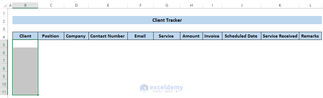
- Choose cell B5 to cell B11.
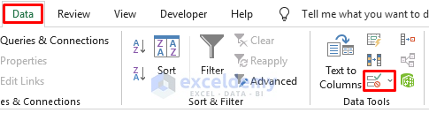
- Click on the Data tab in the ribbon.
- From the Data Tools group, click on Data validation.
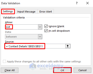
- A Data validation dialog box will appear. From there, click on Settings.
- In the Allow section, click on List.
- In the Source section, click and select the array that contains the information. We take the source from the Contact Details sheet.
- Click on OK.
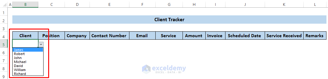
- This will create a drop-down list from there you can choose the client name.
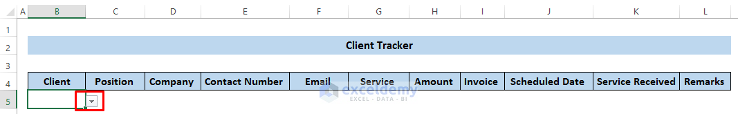
- Click on the drop-down list and choose any of the clients from there.
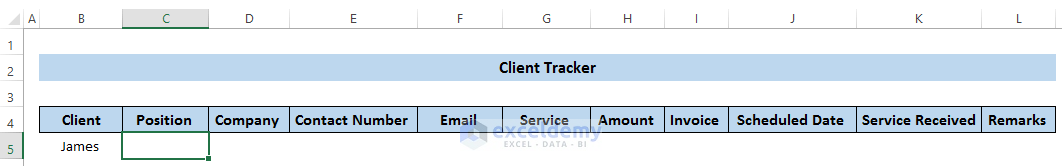
- Click on cell C5.
- Write down the following formula in the formula box:
=IFERROR(VLOOKUP(B5,'Contact Details'!$B$5:$G$11,2,FALSE),0)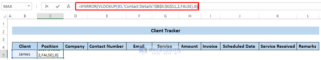
Breakdown of the Formula
- VLOOKUP(B5,’Contact Details’!$B$5:$G$11,2,FALSE): Here, the VLOOKUP function searches the value in cell B5 in the range of B5 to G11 from the worksheet called Contact Details. It will return the second column of that range where B5 is matched. Here, false means you have to have an exact match otherwise it won’t give any result.
- IFERROR(VLOOKUP(B5,’Contact Details’!$B$5:$G$11,2,FALSE),0): The IFERROR function will return zero if the previous function has some error.
- Press Enter to apply the formula.
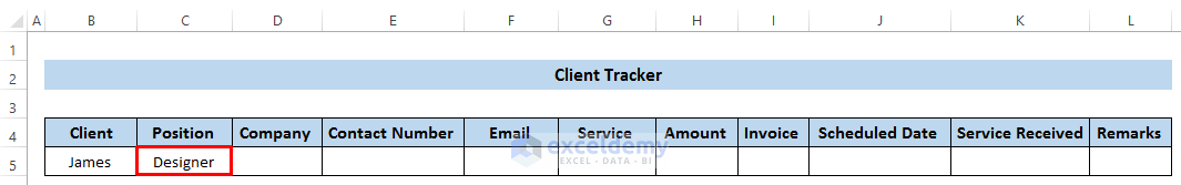
- Changing the client name automatically updates the cell.
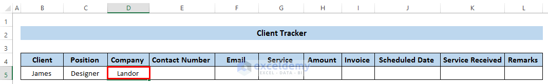
- Click on cell D5.
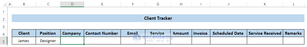
- Write down the following formula in the formula box:
=IFERROR(VLOOKUP(B5,'Contact Details'!$B$5:$G$11,3,FALSE),0)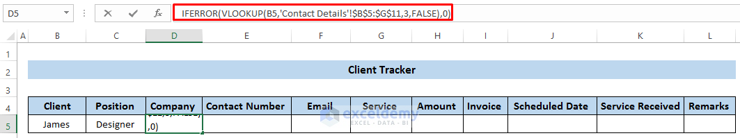
- Press Enter to apply the formula.
- Click on cell E5.
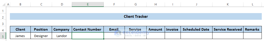
- Write down the following formula in the formula box:
=IFERROR(VLOOKUP(B5,'Contact Details'!$B$5:$G$11,5,FALSE),0)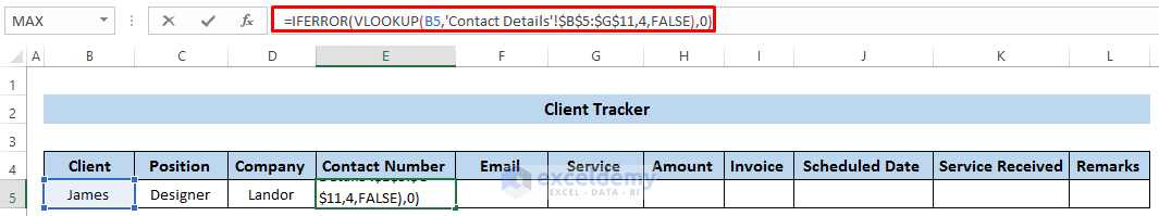
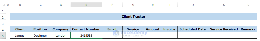
- Press Enter to apply the formula.
- Now, click on cell F5.
- Then, write down the following formula in the formula box.
=IFERROR(VLOOKUP(B5,'Contact Details'!$B$5:$G$11,6,FALSE),0)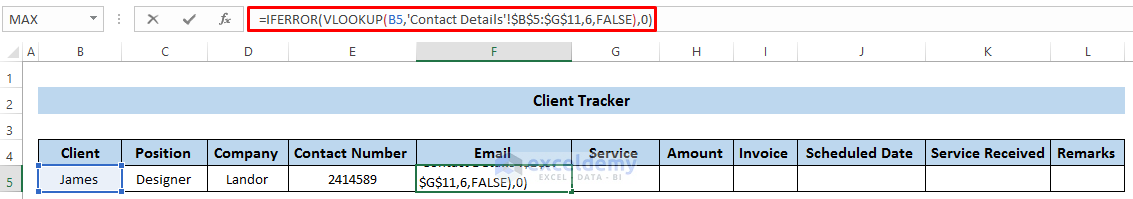
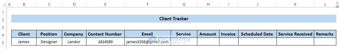
- Press Enter to apply the formula.
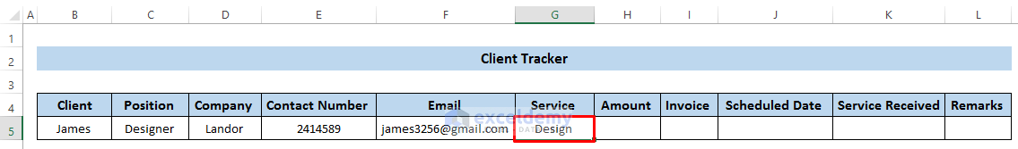
- To get the service of the specific client, click on cell G5.
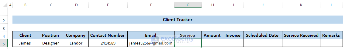
- Write down the following formula in the formula box:
=IFERROR(VLOOKUP(B5,'Service Details'!B5:E11,2,FALSE),0)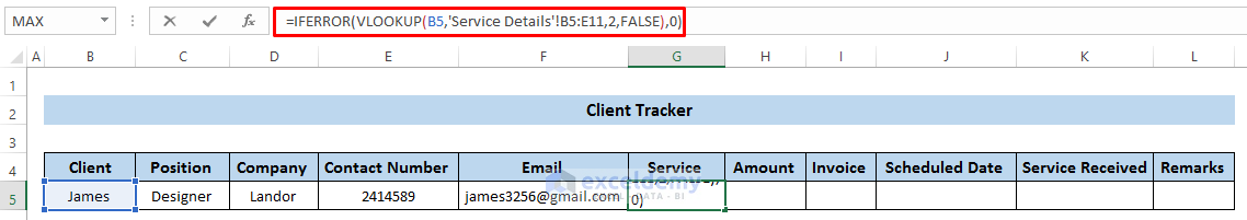
Breakdown of the Formula
- VLOOKUP(B5,’Service Details’!$B$5:$G$11,2,FALSE): Here, the VLOOKUP function searches the value in cell B5 in the range of B5 to G11 from the worksheet called Service Details. It will return the second column of that range where B5 is matched. Here, false means you have to have an exact match otherwise it won’t give any result.
- IFERROR(VLOOKUP(B5,’Service Details’!$B$5:$G$11,2,FALSE),0): The IFERROR function will return zero if the previous function has some error.
- Press Enter to apply the formula.
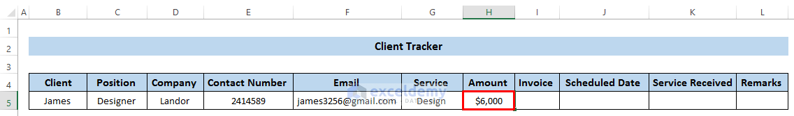
- Click on cell H5.
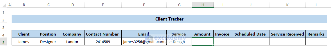
- Write down the following formula:
=IFERROR(VLOOKUP(B5,'Service Details'!B5:E11,3,FALSE),0)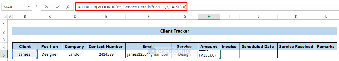
- Press Enter to apply the formula.
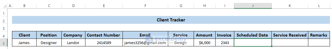
- We need to get the Scheduled Data. So, click on cell J5.
- Write down the following formula:
=IFERROR(VLOOKUP(B5,'Service Details'!$B$5:$F$11,5,FALSE),0)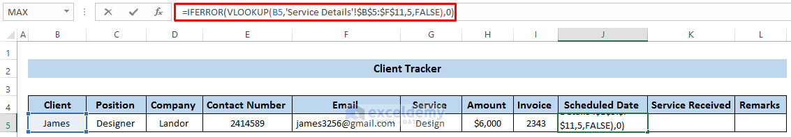
- Press Enter to apply the formula.
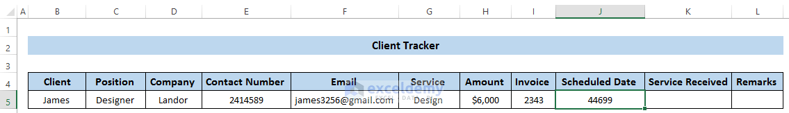
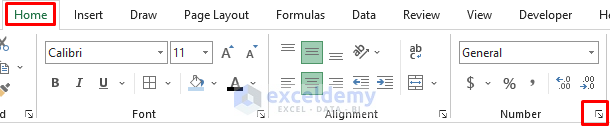
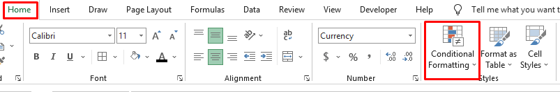
- The scheduled date has appeared in the General format. To change it, go to the Home tab in the ribbon.
- From the Number group, select the little arrow in the bottom right corner. See the screenshot.
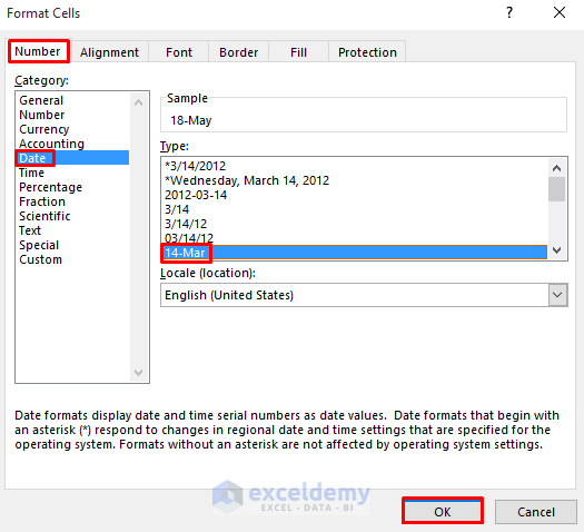
- Format Cells dialog box will pop up.
- Click on the Number command at the top.
- From the Category section, click on Date.
- In the Type section, click on the following pattern: two-digit number and three-letter month.
- Click on OK.
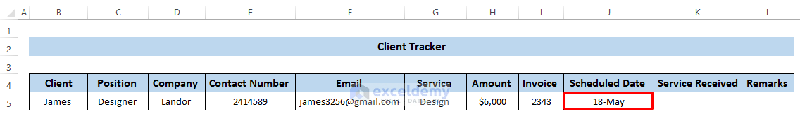
- It will give us the Scheduled Date as the Date format.
- We have a portion called Service Received. It means the time when you receive the service.
- The Remarks section denotes the final outcome of the client whether he/she provides the service in time or not.
- To make Remarks for a specific client, click on cell L5.
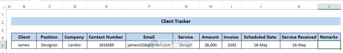
- Write down the following formula:
=IF(J5>K5,"Outstanding",IF(J5=K5,"Good",IF(J5<K5,"Bad")))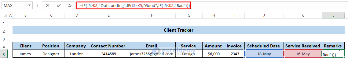
Breakdown of the Formula
- IF(J5>K5,”Outstanding”,IF(J5=K5,”Good”,IF(J5<K5,”Bad”))): This denotes if your client gives the service prior to the scheduled date, he/she will get Outstanding remarks. Then If the client gives the service on time then she/he will get Good remarks. Finally, if the client gives the service after passing the scheduled date, he/she will get Bad remarks.
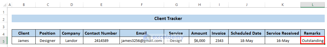
- Press Enter to apply the formula.
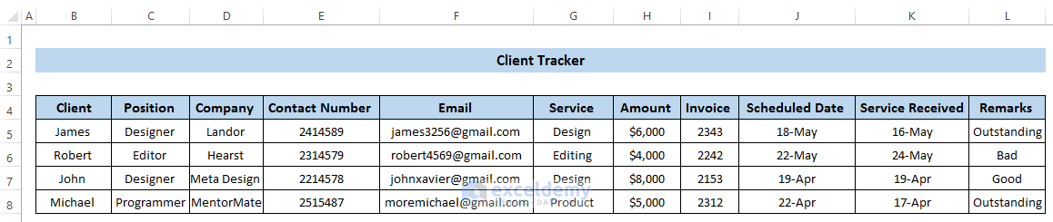
- If we take some other client’s details, we will get the following outcome. See the screenshot.
Step 4 – Make Client Tracker Dynamic
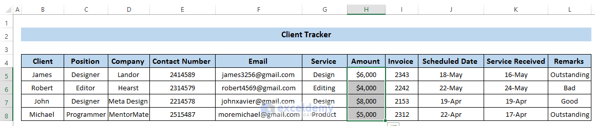
- Choose cells H5:H8.
- Click on Conditional Formatting from the Style group.
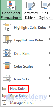
- Click on New Rule.
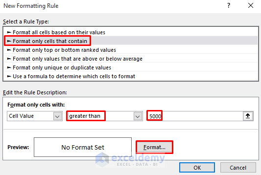
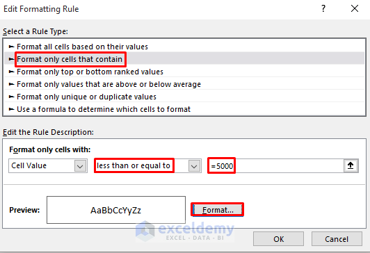
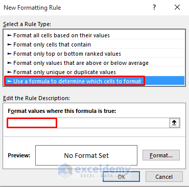
- A New Formatting Rule dialog box will appear.
- Click on Format only cells that contain.
- Set Greater than 5000.
- Click on Format to change the format color.
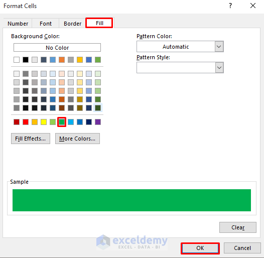
- We put a green color for greater than $5000.
- Click on the Fill command.
- Set Green as your preferred color.
- Click on OK.
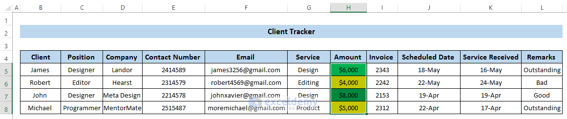
- That will set the amount greater than $5,000 as green.
- Go to Conditional Formatting again.
- In Conditional Formatting, click on New Rule.
- Click on Format only cells that contain.
- Set it to less than or equal to 5000.
- Click on Format to change the format color.
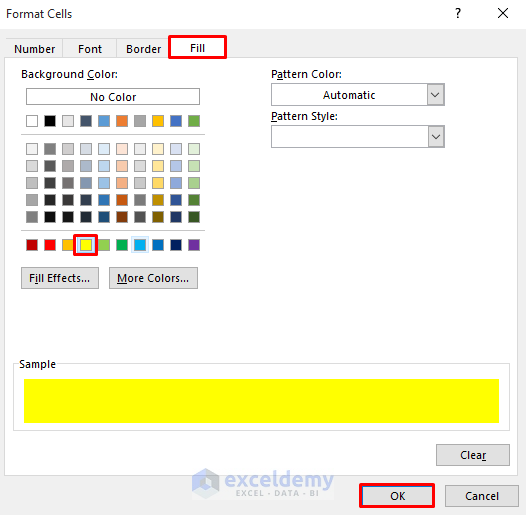
- We put Yellow for less than or equal to 5000.
- Click on the Fill tab.
- Set Yellow as your preferred color.
- Click on OK.
- That will set all the values less than or equal to $5,000 as yellow.
- In terms of remarks, we want to set outstanding remarks as green, good as yellow, and bad as red.
- Select cell range L5:L8.
- Go to Conditional Formatting.
- Choose New Rule.
- Select Use a formula to determine which cells to format.
- Write down the following formula in the box:
=$J5:$J8>$K5:$K8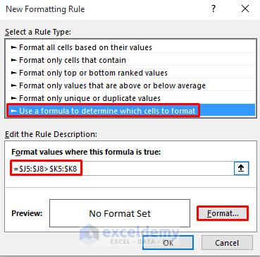
- Click on Format to set the preferred color. Click on the Fill tab.
- Set Green as your preferred color for this condition.
- Click on OK.
Breakdown of the Formula
- $J5:$J8>$K5:$K8: Here, column J denotes the scheduled time, and column K denotes the service received. This condition demonstrates the situation when a client gives their service before the deadline. Another important to remember, if you use the formula in the Conditional Formatting, you don’t need to use the IF function.
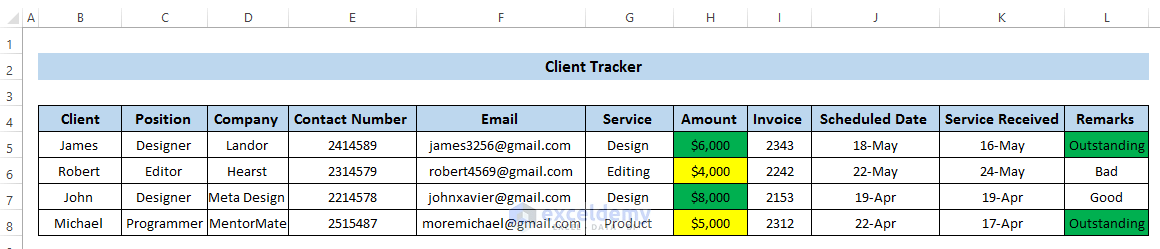
- Finally, It will make Remarks green when some clients give their service before the deadline.
- Next, when clients give their service on time, we want to express their remarks as yellow.
- Make a new Conditional Formatting rule.
- Click on Use a formula to determine which cells to format.
- Write down the following formula in the box:
=$J5:$J8=$K5:$K8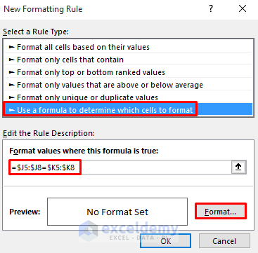
- Set the Format color to Yellow.
- That will set the Remarks which are valid for the formula as yellow.
- Lastly, for those clients who don’t meet the deadline, we want to express their Remarks as Red.
- Make a new Conditional Formatting rule as shown above.
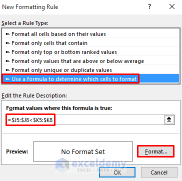
- Click on Use a formula to determine which cells to format.
- Write down the following formula in the box:
=$J5:$J8<$K5:$K8- Then, click on Format to set the preferred color.
- Choose Red and select OK.
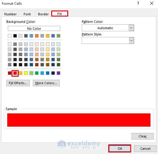
- That will set the Remarks which are valid for the formula as Red.
Read More: How to Make a Sales Tracker in Excel
Download Practice Workbook
Download this practice workbook that can also be used as a template.
Related Articles
- How to Create a Task Tracker in Excel
- How to Create a Daily Task Sheet in Excel
- How to Create a Progress Tracker in Excel
- How to Keep Track of Invoices and Payments in Excel
- How to Create Real Time Tracker in Excel
<< Go Back to Create a Tracker in Excel | Tracker in Excel | Excel Templates
Get FREE Advanced Excel Exercises with Solutions!

This post is a lifesaver! I often struggle to keep my client information organized, and the free template you provided is just what I needed. Thanks for the helpful tips and resources!
Hello,
You are most welcome. Glad to hear that our tutorial is lifesaver to you. Thanks for your appreciation. Keep learning Excel with ExcelDemy!
Regards
ExcelDemy
Hello,
I am business development manager at a small medical laboratory.
I keep back up data on clients that visit our laboratory, as the front desk officer enters manually in a notebook.
I use excel to keep track of clients.
Now I need assistance for a template to be able to design/customize a worksheet that would allow me keep track of daily, weekly and monthly numerical counts of the variuos clients visit to the lab,
i tried something before now, but keep having errors in the formular.
Thank you and hopefully i can get help.
Hello Isukpong Sunday,
Thanks for sharing your situation—it’s great that you’re already using Excel to manage client data! For your needs, I recommend setting up a well-structured Excel template with the following key features:
Client Visit Log Sheet: A table where you enter each client’s visit details (Date, Name, Service Type, etc.).
Summary Dashboard: Use formulas like COUNTIFS and SUMIFS to automatically calculate daily, weekly, and monthly visit counts.
Drop-down Lists: For consistent data entry (like service types or staff names).
Error-Free Formulas: I can help review or fix your formulas to ensure they work properly.
Example Formula – Count Visits on a Specific Date
If your client data is in a table like this:
A (Date) B (Client Name)
2025-03-25 John Doe
2025-03-26 Jane Smith
To count how many clients visited on March 25, 2025, you can use:
=COUNTIF(A2:A100, DATE(2025,3,25))
Or to make it dynamic with a date in cell D1:
=COUNTIF(A2:A100, D1)
If you’d like, I can help you build a complete template with automated summaries for daily, weekly, and monthly tracking. Just let me know the exact fields you want to include!
Looking forward to helping you!
Regards
ExcelDemy
Hello Shamima,
Here is the link (excel Workbook) to what i am doing presently/hope to implement with your assistance.
https://us.docworkspace.com/d/sIAHsx6seqYvZvwY
Isukpong
Best Regards.
Hello Isukpong Sunday,
Thank you for reaching out and sharing your workbook. However, the link you’ve provided opens a file in WPS Office, which we currently don’t support.
Could you please re-upload the file in a compatible format—preferably Excel (.xlsx), using either Google Drive, OneDrive, or simply attaching it via email or another supported link?
Once I have access to the Excel version, I’ll be happy to review it and assist you further.
Regards
ExcelDemy
Hi Shamima,
The link below will open the workbook via google drive.
Thank you for your assistance.
https://docs.google.com/spreadsheets/d/1bahxulEW3DjnmxojBxNr2EZ5U8XLSGfx/edit?usp=drive_link&ouid=106705360010224324373&rtpof=true&sd=true
Hello Isukpong Sunday,
Please share your workbook in our ExcelDemy Forum with proper explanation. We would be happy to help you.
Regards
ExcelDemy