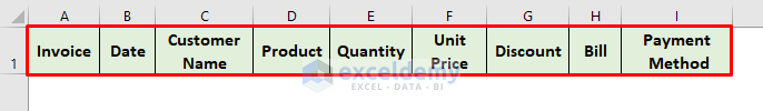
How to Keep Track of Customer Payments in Excel (With Easy Steps)

Step 1: Headline Entry for Customer Payments in Excel

Open an Excel spreadsheet.
Type all the necessary Headline info for the payment data. Look at the picture below for a better understanding.

STEP 2: Input Customer Payments and Apply Data Validation

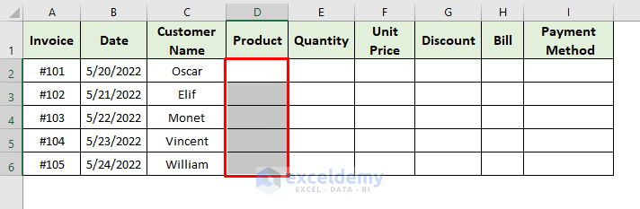
Input the details carefully, one by one. The image below demonstrates how to do so for Invoice Numbers, Payment Dates, and Customer Names.
Select the D2:D6 range.

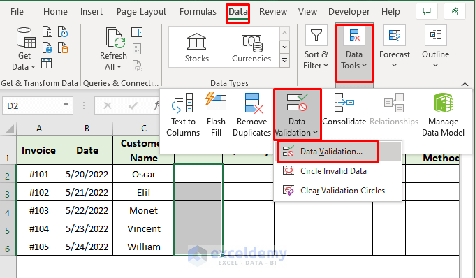
Go to the Data tab and select Data Tools.
Click on the Data Validation button two times, as pictured below.

Choose List from the Allow dropdown menu in the Data Validation dialog box.
Enter Pen Drive,Hard Disk,SD Card,SDHC Card,SDXC Card in the Source box.
Press OK.

Select any cell from the D2:D6 range.
Click on the downward arrow in the right corner to select the option for the Product entry instead of typing over and again.

Step 3: Create Dynamic Payment Details

Input the Quantity, Unit Price, and Discount data.
Copy the following formula for the Bill calculation to cell H2:

=(E2*F2)-G2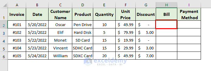

Press Enter and use AutoFill to find out the other Bill values.

NOTE: The Bill becomes dynamic after using the formula. You can update the Unit Price and Discounts at any time, but there’s no need to manually calculate the Bills anymore.

Apply the Data Validation for Payment Methods. See the image below .

Step 4: Compute Total Bill

Select cell H7.
Type the following formula:

=SUM(H2:H6)

Press Enter to return the summation.

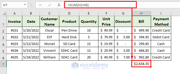
NOTE: The SUM function calculates the total of H2:H6.

Step 5: Generate Dynamic Payments Summary

You can also make a summary based on a specific category apart from Keeping Track of Customer Payments. In this example, we’ll form a Dynamic Summary for the list of Discounted Items and the total count for each Payment Method.

Select cell C10 and enter the following formula:

=IF(G2<>0,D2,"")

Press Enter and use AutoFill to return the list of Discounted Items only.

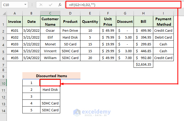
NOTE: The IF function looks for the values in the Discount column and returns that Product name if found. Otherwise, it returns blank.

Choose cell F10 to find the total count for each Payment Method.
Enter the following formula:

=COUNTIF(I2:I6,"Credit Card")

Press Enter to return the result.

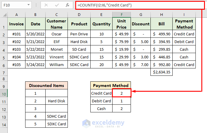
NOTE: Replace Credit Card with Debit Card and Cash in the COUNTIF function argument to find the count for Debit Card and Cash payments, respectively.

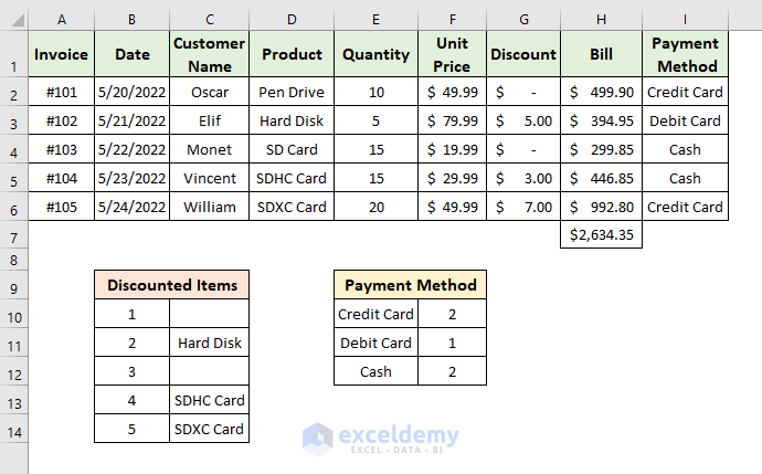
Final Output

The following dataset demonstrates the final output of the Customer Payments tracker in Excel.

Sort and Filter Customer Payments Tracker in Excel

You can also perform the Sort operation on the payment entries or even Filter them. To illustrate, we’ll apply the Filter to view the information details of Credit Card payments.

Steps:

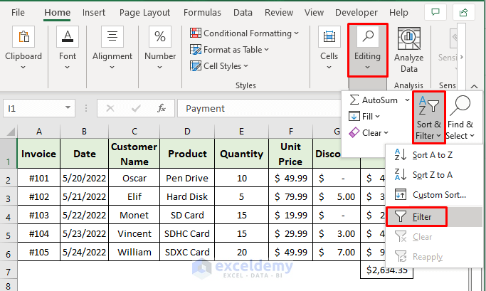
Select any header.
Go to the Home tab and click on the Editing button.
From the dropdown menu, choose the Sort & Filter option followed by Filter.

Select the dropdown icon in the bottom-right corner of the Payment Method header and check Credit Card.
The returned list will show Credit Card payment details only.

Download Template

Download the following template to practice by yourself.

Track Customer Payments.xlsx

<< Go Back to Create a Tracker in Excel | Tracker in Excel | Excel Templates

Get FREE Advanced Excel Exercises with Solutions!

2 Comments

mr1098 Mar 27, 2025 at 9:53 PM

THANK FOR POSTING THIS IT WAS MAJOR HELP TO ME SINCE IM NOT EXCEL SKILL FLUENT. YOU A MAJOR BLESSING!!!
- Reply
  Shamima Sultana Mar 28, 2025 at 11:47 AM
  
  Hello Mr1098,
  
  You are most welcome. Thanks for your feedback and appreciation. Glad to hear that our post helped you a lot. Keep exploring Excel with ExcelDemy!
  
  Regards
  ExcelDemy