Method 1 – Create a Daily Task Sheet with a Drop-Down List
Steps:
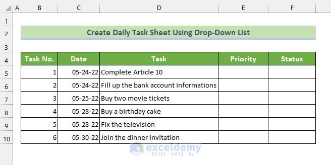
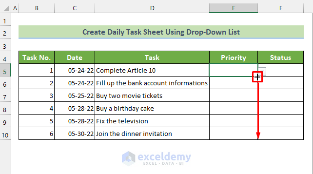
- Prepare your daily task sheet table with column headings. To automate the priority and status of individual tasks:
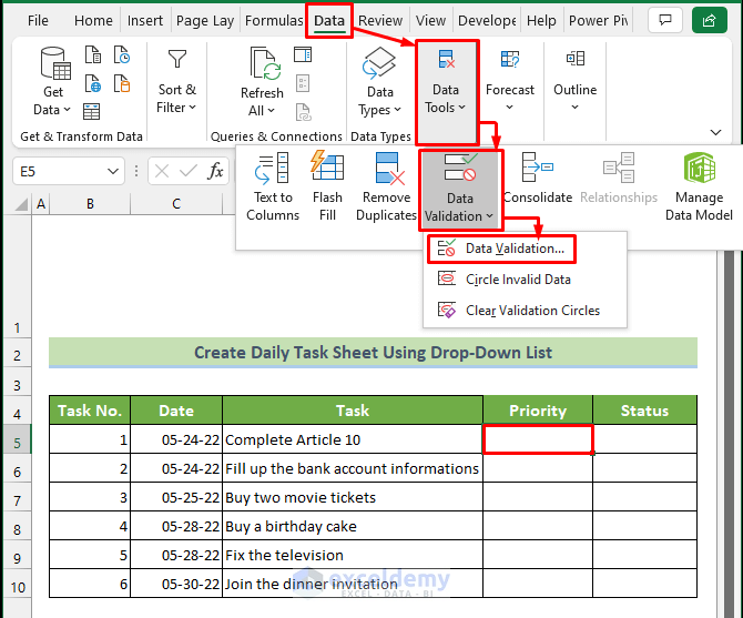
- Click the cell in which you want to place the priority of the task. Go to the Data tab >> Data Tools >> Data Validation >> Data Validation…
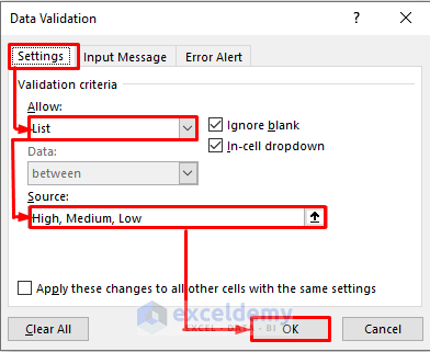
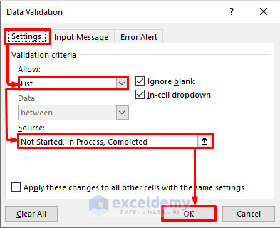
- In the Data Validation window, select Settings.
- In Allow, choose List.
- Enter the priority options you want to select automatically in the Source text box. Separate every option by a comma(,).
- Click OK.
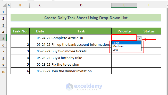
- Click the drop-down arrow in E5 to select a priority option.
- Drag down the Fill Handle to see the result in the rest of the cells.
- Set data validation in the Status column. Enter the status options in the Source text box.
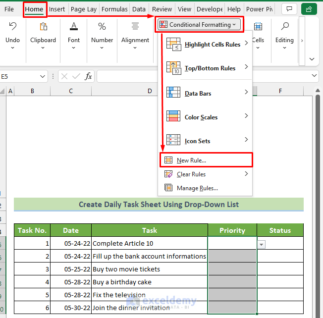
- To format the priority options, select the priority cells >> go to the Home tab >> click Conditional Formatting >> click New Rule…
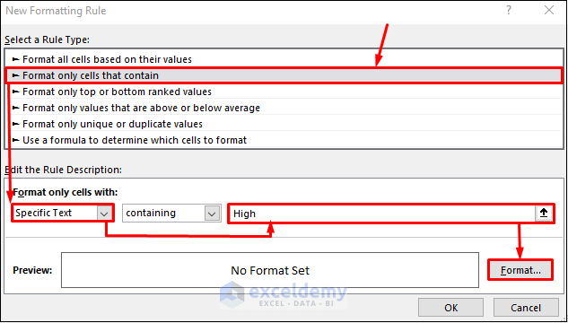
- In the New Formatting Rule window, choose Format only cells that contain in Rule Type.
- In Format only cells with:, select Specific text.
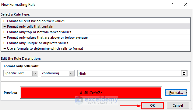
- Set the format to high priority: enter High in the right side text box.
- Click Format.
- In the Format window, in Fill, choose a color.
- Click OK.

- In the New Formatting Rule window, click OK.
- Set formats for medium and low priority tasks.
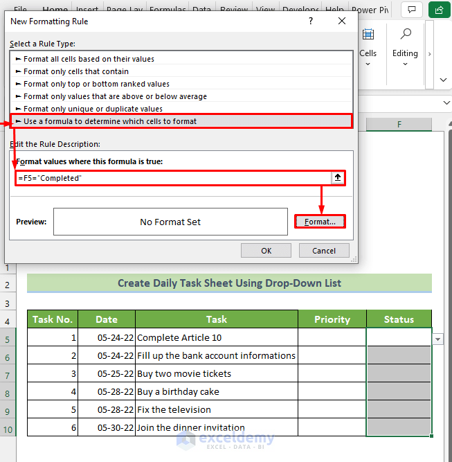
- You can also set the format of the Status column: select the status cells >> go to the Home tab >> click Conditional Formatting >> click New Rule…
- In the New Formatting Rule window, choose Use a formula to determine which cells to format in Rule Type.
- Enter equal sign (=) in the formula text box to enter a formula. The format is set to a completed status: enter “Complete”.
- Click Format.
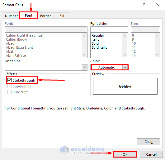
- In the Format Cells window, go to the Font tab.
- Check Strikethrough. You can also change the format of font color and change the fill color in Fill.
- Click OK.
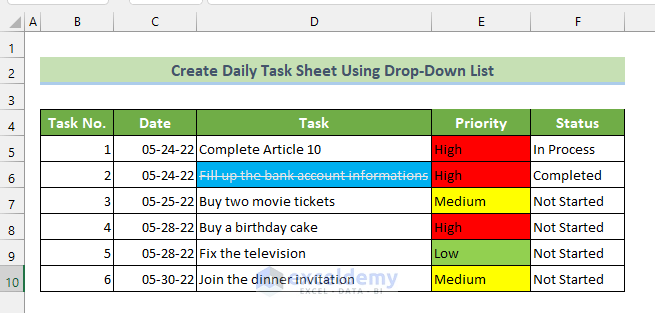
This is the output.
Read More: How to Create Real Time Tracker in Excel
Method 2. Create a Daily Task Sheet with a Checkbox
Steps:
- Follow the first eleven steps in Method 1.
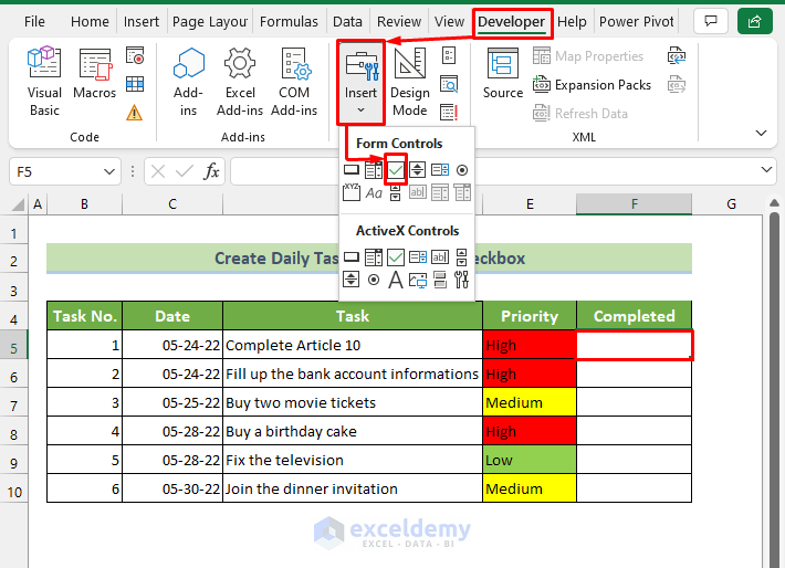
- Add checkboxes: select the Completed column >> Go to the Developer tab >> click Insert >> click the Checkbox icon.
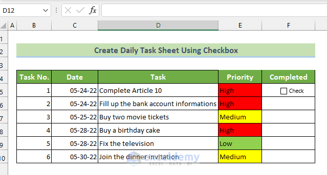
- Drag and move the checkbox inside the cell.
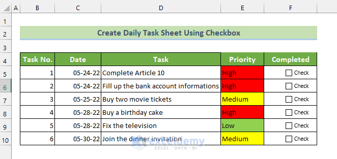
- Repeat the process for all other status cells. Checkboxes will be displayed in all cells of the Completed column.
- To remove the text Check, right-click the checkbox and choose Edit Text.
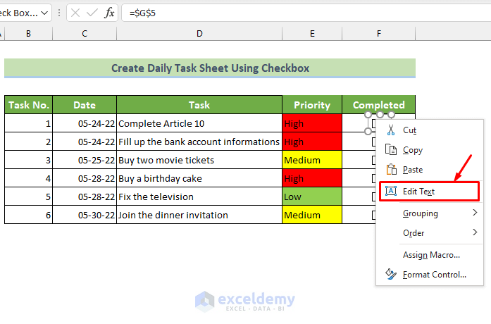
- Delete all text characters. Repeat the process for every checkbox. Only the checkbox icon will be displayed.

- To add formatting to the checkboxes, extract their values.
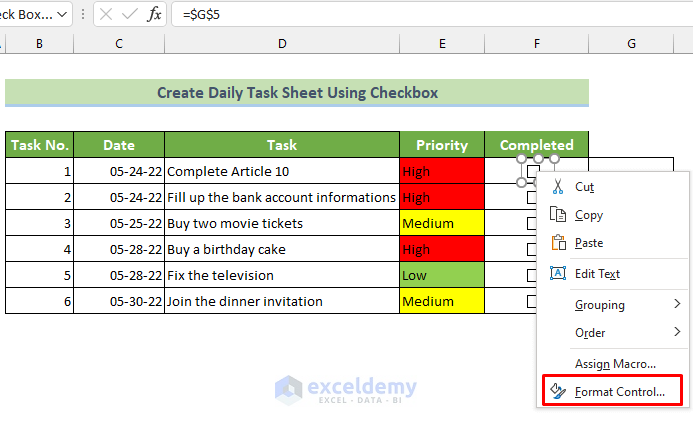
- Right-click the checkbox and choose Format Control…
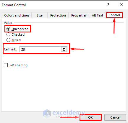
- In the Format Control window, choose the Control tab.
- Make sure the value is selected as Unchecked.
- Link the cell to place the extracted value, here G5.
- Click OK.
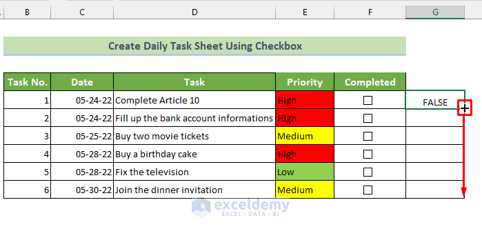
- The checkbox will display FALSE when unchecked and TRUE when checked. Drag the fill handle to copy the format to the cells below.
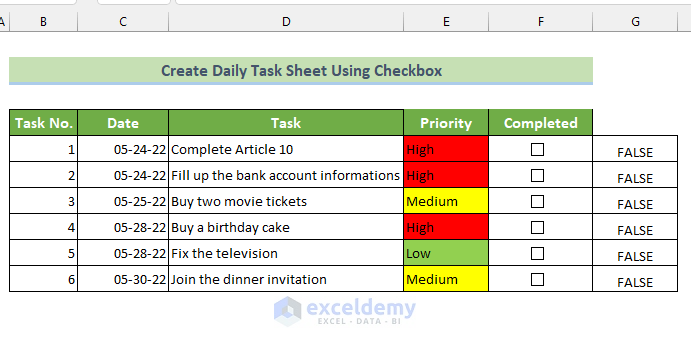
- Every cell in the Completed column has a value beside the checkboxes. All values are FALSE as checkboxes are unchecked.
- Format the completed tasks.
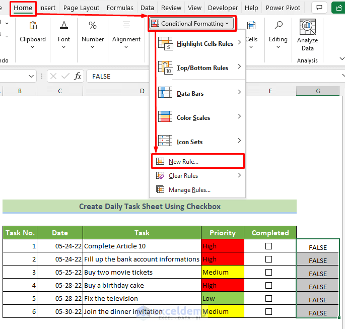
- Select D5:G10 >> go to the Home tab >> click Conditional Formatting >> click New Rule…
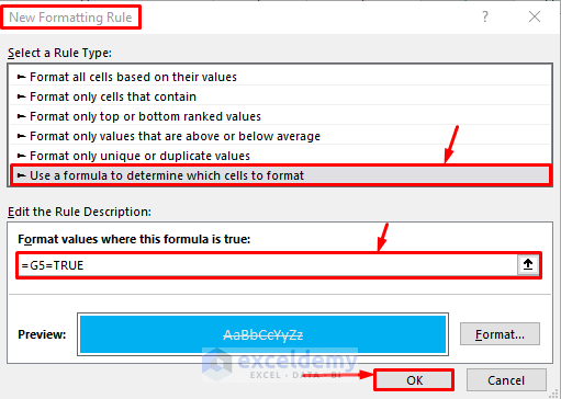
- In the New Formatting Rule window, choose Use a formula to determine which cells to format in Rule Type.
- Enter equal sign (=) in the formula text box to enter a formula. The format is set to completed status, which is determined by the checked checkbox: enter TRUE.
- Click Format.
- In the Format Cells window, go to the Font tab.
- Check Strikethrough option. You can also change the format of font color and fill color in Fill.
- Click Ok.
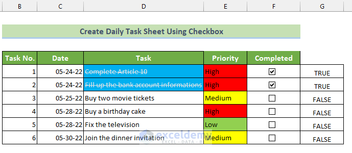
The daily task sheet displays checkboxes. If you click the checkbox, TRUE will be returned.
Read More: How to Create a Progress Tracker in Excel
Method 3 – Prepare a Double-Click-Enabled Daily Task Sheet
Steps:
Follow the first 11 steps in Method 1 to automate the task priority.
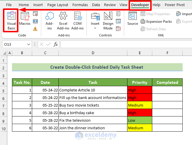
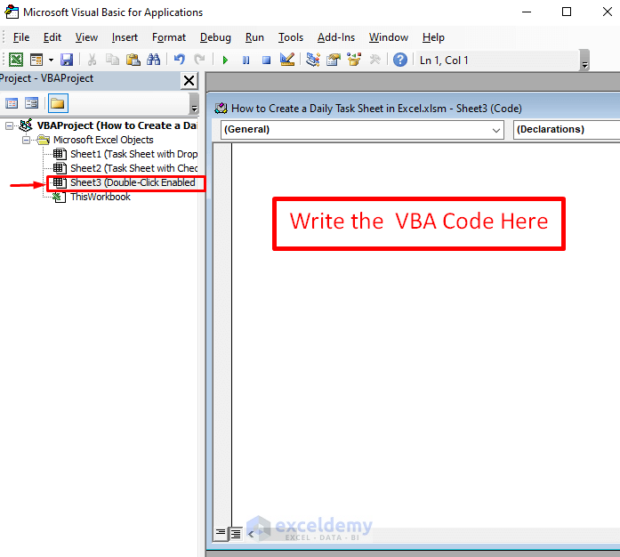
- Go to the Developer tab >> Visual Basic.
- In the Microsoft Visual Basic for Applications window, click Sheet 3 and enter the following code:
Private Sub Worksheet_BeforeDoubleClick(ByVal Target As Range, Cancel As Boolean)
Cancel = False
    If Target.Row >= 5 And Target.Row <= 10 And Target.Column = 6 Then
    Cancel = True
        If Cells(Target.Row, Target.Column) <> Range("G5").Value Then
            Cells(Target.Row, Target.Column).Value = Range("G5").Value
        Else: Cells(Target.Row, Target.Column).Value = "No"
        End If
    End If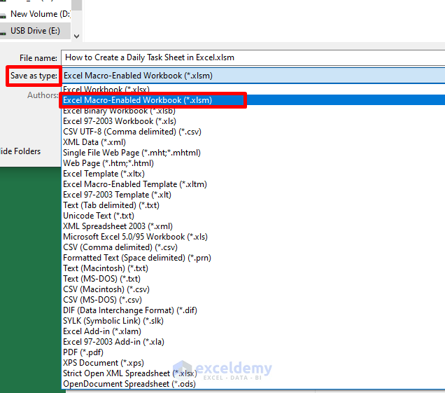
End Sub- Save the workbook as an Excel-Macro Enabled Workbook (.xlsm).
- Close it and reopen it again. The macro is enabled.
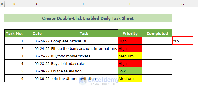
- Enter YES in G5.
- By double-clicking a cell, between row 5 and row 10 in column 6 (declared in the code), YES will be displayed.
- Another double-click will toggle the value to NO.
- Fill all the cells by toggling double-click.
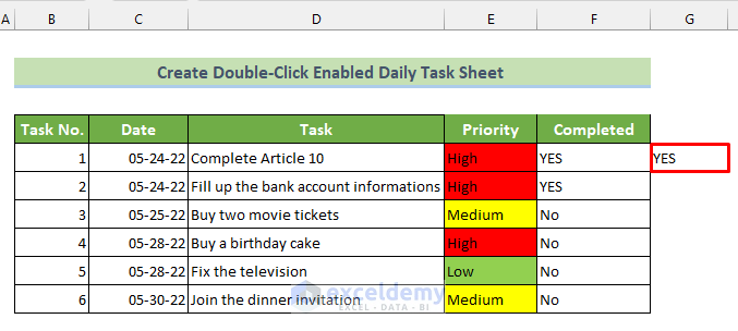
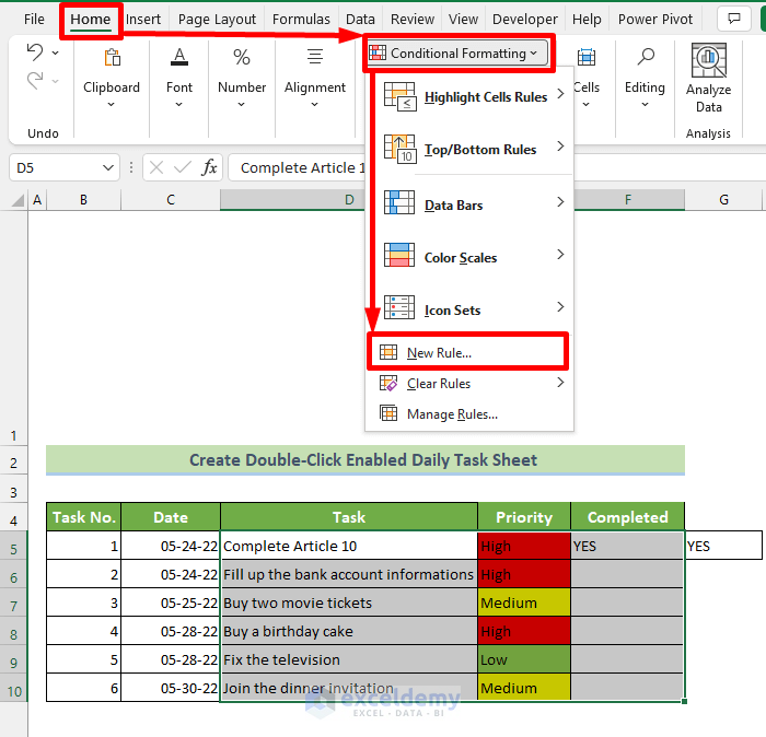
- Apply conditional formatting: select the cells >> go to the Home tab >> click Conditional Formatting >> click New Rule….
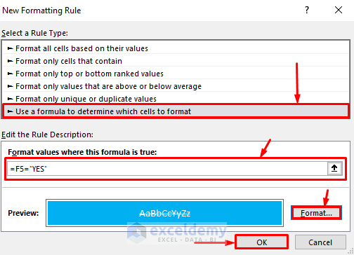
- Select the Rule Type as Use a formula to determine which cells to format >> in the formula text box, write =F5=”YES” >> click Format >> Check Strikethrough in Font and in Fill, choose a color.
- Click OK.
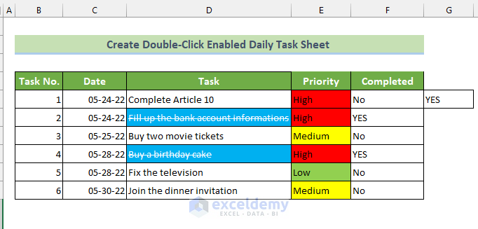
This is the output.
Read More: How to Create a Task Tracker in Excel
Points to Remember
- Do not use absolute cell reference in conditional formatting.
Download the template and practice.
Related Articles
- How to Keep Track of Clients in Excel
- How to Keep Track of Invoices and Payments in Excel
- How to Keep Track of Customer Payments in Excel
- How to Keep Track of Customer Orders in Excel
- How to Make a Sales Tracker in Excel
<< Go Back to Create a Tracker in Excel | Tracker in Excel | Excel Templates
Get FREE Advanced Excel Exercises with Solutions!
