Functions Used in This Article
The COUNTIFS Function:
This function counts cells that match multiple criteria. The syntax of the COUNTIFS function is as follows.
=COUNTIFS (range1, criteria1, [range2], [criteria2], …)
- range1 – The 1st range to evaluate.
- criteria1 – The criterion to use on the 1st range.
- range2 [optional]: The 2nd range, acts just like range1.
- criteria2 [optional]: The criterion to use on the 2nd range. This function allows a maximum of 127 ranges and criteria pairs.
The TEXTJOIN Function:
This function joins text values with a delimiter. The syntax of the TEXTJOIN function is as follows.
=TEXTJOIN (delimiter, ignore_empty, text1, [text2], …)
- delimiter: The separator between texts that the function going to combine.
- ignore_empty: This argument specifies if the function ignores the empty cells or not.
- text1: 1st text value (or range).
- text2 [optional]: 2nd text value (or range).
The MATCH Function:
This function gets the position of an item in an array. The syntax of the MATCH function is as follows.
=MATCH (lookup_value, lookup_array, [match_type])
- lookup_value: The value to match in lookup_array.
- lookup_array: A range of cells or an array reference.
- match_type [optional]: 1 = exact or next smallest, 0 = exact match, -1 = exact or next largest. By default, match_type=1.
The INDEX Function:
This function gets values in a list or table based on location. The syntax of the INDEX function is as follows.
=INDEX (array, row_num, [col_num], [area_num])
- array: Range of cells, or an array constant.
- row_num: The row position in the reference.
- col_num [optional]: The column position in the reference.
- area_num [optional]: The range in reference that should be used.
The IFERROR Function:
This function traps and handles errors. The syntax of the IFERROR function is as follows.
=IFERROR (value, value_if_error)
- value: The value, reference, or formula to check for an error.
- value_if_error: The value to return if an error is found.
The SEARCH Function:
This function gets the location of text in a string. The syntax of the SEARCH function is as follows.
=SEARCH (find_text, within_text, [start_num])
- find_text: This argument specifies which text to find.
- within_text: This specifies where to find the text.
- start_num [optional]: With this, you will specify- from which position in the text string you will count the position of the specified text. Optional and defaults to 1 from left.
How to Return a Value in Excel If a Cell Contains Text from List: 5 Methods
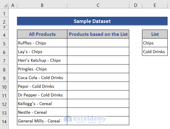
We have a list of products that fall in one of three categories: Chips, Cold Drinks, and Cereals. The column All Products contains the name and categories of the beverages linked together. Two of these categories, Chips and Cold Drinks, are also in the List column. We will return a list of the products that satisfy the List criteria.
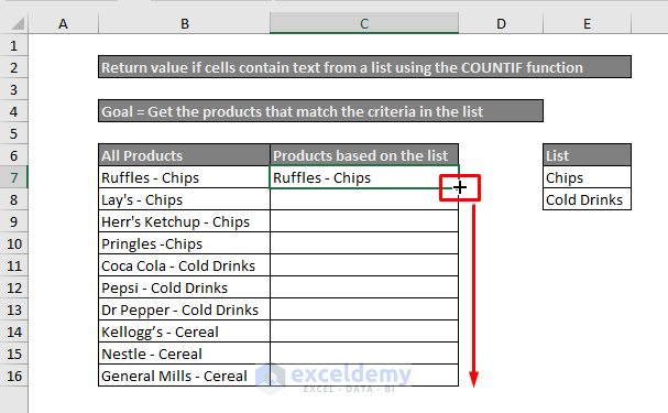
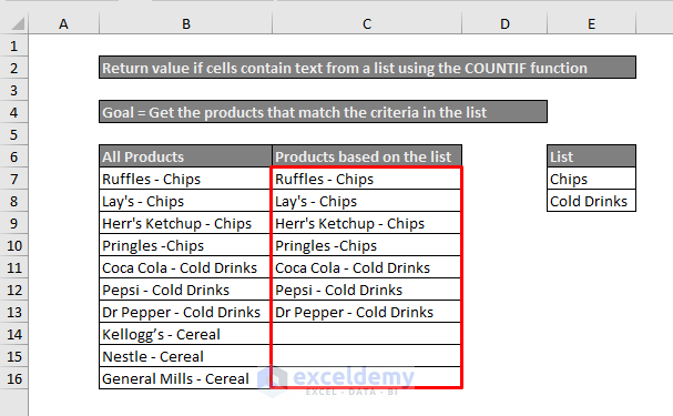
Method 1 – Combine COUNTIF, IF, and OR Functions to Return a Value If a Cell Contains Text from a List
We have fetched the cell values of the Products that matched the List column criteria and showed them to the Product based on that list column.
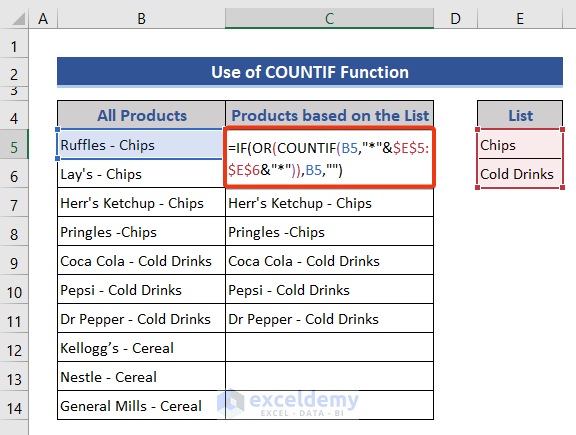
- Use the following formula:
=IF(OR(COUNTIF(B5,"*"&$E$5:$E$6&"*")),B5,"")
Formula Breakdown:
- The Asterisk sign (*) is a wildcard character. It searched for “Chips” and “Cold Drinks” substrings within Cell B5 which is “Ruffles – Chips” string.
- The COUNTIF function returned one for every substring match. As “Chips” is found in Cell B5, it returns {1:0}.
- The OR function returns a TRUE value if any of the arguments are TRUE. In this case, one (1)= TRUE.
- As the IF function’s value is TRUE, it returns the first argument which is the desired output.
- Final Output: Ruffles – Chips
Note:
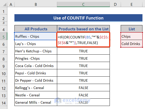
You can change the cell output by modifying the last two arguments of the IF function:
=IF(OR(COUNTIF(B5,"*"&$E$5:$E$6&"*")),TRUE,FALSE)
Tip/Reminder: Method 1 works fine for short lists, but keep in mind it has a 255-character limit. If your list is longer, the formula may stop working without a clear error. In that case, it’s better to use an array-based approach (e.g., with SEARCH + INDEX/MATCH) or move to the TEXTJOIN method, which handles long lists more reliably.
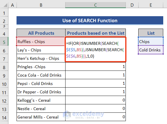
Method 2 – Use IF, OR, ISNUMBER, and SEARCH Functions to Return a Value with Multiple Conditions
We have fetched the cell values of the Products that matched the List column criteria and showed them to the Product based on that list column.
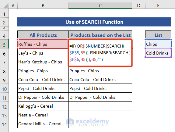
- The formula is as follows:
=IF(OR(ISNUMBER(SEARCH($E$5,B5)),ISNUMBER(SEARCH($E$6,B5))),B5,"")
Formula Breakdown:
=IF(OR(ISNUMBER(SEARCH($E$5,B5)),ISNUMBER(SEARCH($E$6,B5))),B5,"")
The SEARCH function searched the values of the List column in Cell B5. For “Chips” it returned 11 which is the starting position of the substring. For Cold Drinks, it returned an error.
=IF(OR(ISNUMBER(11),ISNUMBER(SEARCH(#VALUE))),B5,"")
The ISNUMBER function converted 11 into TRUE value and the error into FALSE value.
=IF(OR(TRUE,FALSE)),B5,"")
The OR function returns a TRUE value if any of the arguments are TRUE. As there is a TRUE argument, it also returns the TRUE value in this case.
=IF(TRUE, "Ruffles - Chips","")
As the IF function’s value is TRUE, it returns the first argument which is the desired output.
Final Output: Ruffles – Chips
Note:
- You can modify the output through the final two arguments:
=IF(OR(ISNUMBER(SEARCH($E$5,B5)),ISNUMBER(SEARCH($E$6,B5))),1,0)
- This is not an array formula, so drag the Fill Handle to fill the column.
- For case-sensitive searches, use the following formula:
=IF(OR(ISNUMBER(FIND($E$5,B5)),ISNUMBER(FIND($E$6,B5))),B5,"")
Method 3 – Use TEXTJOIN to Return a Value in Another Cell If a Cell Has a Text from a List
We have fetched the cell values from the LIST column where they matched with the Product and showed them as a result.
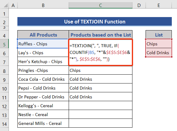
- The formula is as follows:
=TEXTJOIN(", ",TRUE,IF(COUNTIF(B5,"*"&$E$5:$E$6&"*"), $E$5:$E$6,""))
Formula Breakdown:
=TEXTJOIN(", ",TRUE,IF(COUNTIF(B5,"*"&$E$5:$E$6&"*"),$E$5:$E$6,""))
Here, the Asterisk sign (*) is a wildcard character. It searched for “Chips” and “Cold Drinks” substring within Cell B5 which is “Ruffles – Chips” string.
TEXTJOIN(", ",TRUE,IF(COUNTIF("Ruffles - Chips",*Chips*, *Cold Drinks*),$E$5:$E$6,""))
The COUNTIF function returned one for every substring match. As “Chips” is found in Cell B5, it returns {1:0}.
TEXTJOIN(", ",TRUE,IF({1;0},$E$5:$E$6,""))
The IF function returned only the “Chips” value as only the first value of its argument was one = True.
TEXTJOIN(", ",TRUE,{"Chips";""})
The TEXTJOIN function didn’t do anything here as only one value from the List was matched. If there were many values to match, it would have returned all of them with commas (,) between them as a separator.
Final Output: Chips
Method 4 – Use an INDEX-MATCH Formula to Return a Value If a Cell Contains Specific Text
We have fetched the cell values from the LIST column where they matched with the Product and showed them in the result column.
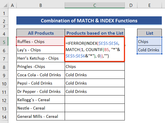
The formula is as follows:
=IFERROR(INDEX($E$5:$E$6, MATCH(1, COUNTIF(B5, "*"&$E$5:$E$6&"*"), 0)),"")
Formula Breakdown:
=IFERROR(INDEX($E$5:$E$6,MATCH(1,COUNTIF(B5,"*"&$E$5:$E$6&"*"),0)),"")
Here, the Asterisk sign (*) is a wildcard character. It searched for “Chips” and “Cold Drinks” substring within Cell B5 which is “Ruffles – Chips” string.
IFERROR(INDEX($E$5:$E$6,MATCH(1,COUNTIF("Ruffles - Chips",*Chips*,*Cold Drinks*),0)),"")
The COUNTIF function returned one for every substring match. As “Chips” is found in Cell B5, it returns {1:0}.
IFERROR(INDEX($E$5:$E$6,MATCH(1,{1;0}),0)),"")
The MATCH function returned one as there is only one value “Chips” that matched.
IFERROR(INDEX($E$5:$E$6,1),"")
The INDEX function returned “Chips” as it was the value in the List array.
IFERROR("Chips","")
Here, the IFERROR function is used to handle the error that will occur if there are no matches.
Final Output: Chips
Method 5 – Apply the EXACT Function with IF and TEXTJOIN
We showed all the match values in a single cell.
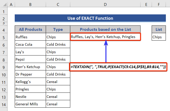
- The formula is as follows:
=TEXTJOIN(", ",TRUE,IF(EXACT(C5:C14,$F$5),B5:B14,""))
Formula Breakdown:
EXACT(C5:C14,$F$5)
This part checks which values of the Range C5:14 match with Cell F5 and return TRUE and FALSE.
IF(EXACT(C5:C14,$F$5),B5:B14,"")
This part returns the names for which we get TRUE.
TEXTJOIN(", ",TRUE,IF(EXACT(C5:C14,$F$5),B5:B14,""))
This joins all the names with a comma after each name.
Quick Notes
For array formulas, press Ctrl + Shift + Enter instead to apply the formula. If you are an Office 365 user, then you can apply them by pressing Enter.
Download the Practice Workbook
<< Go Back to Text | If Cell Contains | Formula List | Learn Excel
Get FREE Advanced Excel Exercises with Solutions!

I have a question , I have a column with string of texts (sheet1) and I want to lookup to a list of texts (Sheet2) to find any matching words and return the matching words in sheet 1.
I.e sheet1
Column A
Chocolate lava cake
Sheet 2
Column A
Lava cake
Strawberry drink
Banana muffin
Result sheet 1
I.e
Column A
Chocolate lava cake
Column B
Lava cake
Would you be able to help me ?
Dear Ashiliah
Thank you for your comment.
Let me now show you how you can solve your problem.
Based on your description I’ve created the dataset.
Here, you can see in the following picture that we have Chocolate lava Cake in cell A5. we keep this in Sheet1.
After that, in Sheet2, we have Lava cake, Strawberry drink, and Banana muffin in cells A5, A6, and A7 respectively.
Next, we will type the following formula in cell B5 of Sheet1.
=TEXTJOIN(", ", TRUE, IF(COUNTIF(A5, ""&Sheet2!A5:A6&""),Sheet2!A5:A6, ""))After that, press ENTER.
As a result, you can see Lava cake in column B of sheet1.
I hope you understand the solution. If you have any problems you can always let us know in the comment section.
Regard
Afia Aziz kona
I’m trying to use “3. Using the TEXTJOIN function” above in Excel 365, but it persistently returns #NAME? error on everything I try. Also tried Ctrl+Shift+Enter, even though not required in Excel 365
My formula is:
“=TEXTJOIN(“, “, TRUE, IF(COUNTIF($J$2,“*”&$F$2:$F$4&”*”), $F$2:$F$4, “”))”
Problem appears to be with the “*,” because the cell array only works:
“=TEXTJOIN(“, “, TRUE, IF(COUNTIF($J$2,“*”&{“NCM”;”BV”;”4+8″}&”*”), $F$2:$F$4, “”))”
But when I include the “*” I get:
“=TEXTJOIN(“, “, TRUE, IF(COUNTIF($J$2,{#NAME?;#NAME?;#NAME?}), $F$2:$F$4, “”))”
Any idea what is causing the #NAME? result?
Dear W
Thank you for your comment.
Let me show you that your formula works properly.
Here, I created the List column including cells F2:F4.
Along with that, I created a Product column that includes cell J2.
Here, as I do not know your actual dataset, I take List and Product according to my choices, however, the cells are the same as your description.
Further, I type the following formula in cell B4.
=TEXTJOIN(", ", TRUE, IF(COUNTIF(J2,"*"&$F$2:$F$4&"*"), $F$2:$F$4, ""))This is the same formula you mentioned in the comment.
After that, I press ENTER.
As a result, you can see the result in cell B4.
Therefore, the formula works properly.
I hope that your problem will be solved now.
If you face any further problems, please share your Excel file with us in the comment section.
Regards
Afia Aziz Kona
Hi,
When I try to use the formula COUNTIF, the CRITERIA picks up only the first name in the list range and ignores rest of the list. Can you please guide me why?
I am having this issue as well, following the steps of it and criteria only picks the first cell. To make it clearer, in explanation it says the formula searches for “Chips” and “Cold Drinks” but when you apply the formula in excel it only searches for “Chips”. What am i missing i couldnt understand ?
Hi AHMETCAN,
Thanks for your comment. I am replying to you on behalf of Exceldemy. To get all the desired values from the list, you need to drag the Fill Handle down to copy the formula. You can follow the steps below to get all the values.
STEPS:
1. Firstly, select Cell C7 and type the formula below:
=IF(OR(COUNTIF(B7,"*"&$E$7:$E$8&"*")),B7,"")2. Press Enter to see the result.
3. Thirdly, move the cursor to the bottom right corner of Cell C7, it will turn into a small black plus sign.
4. Now, drag the Fill Handle down to Cell C16.
5. Finally, you will see results like the picture below.
I hope this will help you to solve your problems. Please let us know if you have other queries.
Thanks!
Hi SANKARSHAN
Generally, you can set one CRITERIA when you apply only COUNTIF Function.
However, if you use a formula that has multiple functions, you can set multiple criteria.
Let me show you an example.
● Suppose you have a set of fruits. You want to count the instances when the fruit is either Mango or Apple.
● Go to D5 and write down the following formula
=COUNTIF(B4:B15,B4)+COUNTIF(B4:B15,B5)Here, Excel will count the instances when the criteria is Mango or Apple from the same range B4:B15.
● Now, press ENTER to get the output.
I hope it helps.
You can also check the following articles to internalize the concept.
● COUNTIF with Multiple Criteria in Different Columns in Excel
● COUNTIFS with Multiple Criteria (5 Easy Methods)
Thank you.
Hello AFIA, I’ve used exact example and used even the same cells and formula. But it still results in #Name error. What could be the reason?
Hello ANANDA,
#NAME error mostly occurs when you misspell the function name. Please check if you have used the correct spelling of the function.
There can be another reason behind this. If you notice you will see that W had fixed the Cell value in the COUNTIF function which is used as the range. Try to use only Cell J2 as the range without making it a fixed range.
If you are using Excel 365 version you only need to press Enter after inserting this array formula. But, for previous versions press Ctrl+Shift+Enter.
I hope that your problem will be solved now.
If you face any further problems, please share your Excel file with us in the comment section.
Regards
Arin Islam
Hello,
Thanks for the tutorial. I have a question. What if the list of words are in different cases in different cells. For example in some cells “Chips” is given as “chips” with lower case “c”.
In such cases how to return all values irrespective of case
Hi Anna!
You wanted to say what will happen if we input the same word with Upper and Lower case. The fact is Excel counts Upper and Lower case characters as the same. So you won’t have any issues. Even then I am showing one way to make your data to proper format first. Then, use the formatted text in the required formula.
=PROPER(B5)If the search cell has multiple values from the criteria, what changes do you need to make to the formula?
Hello Tejas,
If the search cell has multiple criteria, you can use the following formula:
=TEXTJOIN(“, “, TRUE, IF(ISNUMBER(SEARCH($E$4:$E$5, B4)), $E$4:$E$5, “”))
It checks if any of the values in the criteria range are found within the text in cell B4. The SEARCH function identifies the presence of these values, and ISNUMBER confirms their existence. The IF function returns the matching values, while TEXTJOIN concatenates them into a single string, separated by commas, ignoring empty results. This allows multiple matches to be displayed in one cell.
Regards
ExcelDemy
These don’t work on anyone else’s machines but your own apparently. I recreated the example from Mursalin’s reply (cell by cell) and only the first instance of the formula works (in cell C7). The formula is copied as described to the rest of the cells in column c (C7:C16). None of the other cells are populating.
Hello Brian,
If the formula only works in C7 but not in the other cells (C8:C16), please make sure you are using absolute references correctly in your formula, and that the ranges are set properly when you copy down. Sometimes, copying a formula down can change relative references, which may cause the formula not to work as expected.
Also, double-check that your list/range names are consistent and that there are no hidden spaces or formatting issues in your data.
If you still face issues, please share the exact formula you are using, so the community can help you debug it step by step!
Regards
ExcelDemy
There’s a slight problem – you should mention that method 1 works only on ranges below 255 characters, with your example it works fine, but with longer lists you might be stuck without knowing where’s the problem instead moving to textjoin method which solves it.
Hello Kerebron,
Thank you for pointing this out! Method 1 has the 255-character limitation when handling longer lists, which can cause unexpected issues. For larger ranges, switching to the TEXTJOIN-based approach is indeed the safer and more flexible solution. We highlighted this in the explanation so others don’t run into the same problem.
Regards,
ExcelDemy