A crucial ability, effective money usage becomes even more crucial in terms of various trading, transactions, budget etc. In this article, we’ll walk you through the process of how to use money in Excel.
Money Management
The art of managing your finances includes investing and using your hard-earned cash. Everyone requires this essential talent to succeed in life. For various transactions, budget trading, understanding of money management is a requirement. One could experience a terrible loss if they don’t have a thorough comprehension of this. The maximum loss or risk that can be borne can be determined using the money management sheet for trading. Learn about this if you plan to stay in the trading industry for a long time. Because luck or arbitrary choices will eventually run out because they only function temporarily.
Procedures to Use Money in Excel: Step-by-Step
In this article, we will demonstrate how to use money in Excel in terms of trading. Here, we will consider four main key factors to use money in terms of trading and these factors are given below.
- Key Factors.
- Trade Date.
- Potential Trades (Qty Calculation)
- The Actual Trades
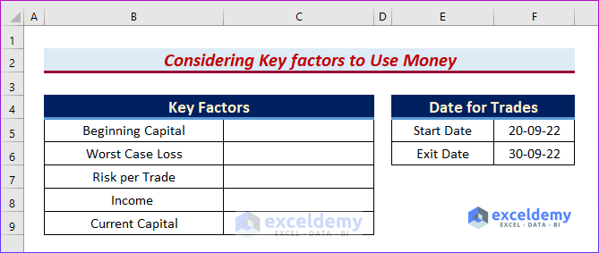
Step 1: Considering Key factors to Use Money in Terms of Trading
In this initial step, we will include the crucial elements of trading money management.
- To begin with, type the following key factors:
- “Beginning Capital” → the initial investment from an individual to start this trading.
- “Worst Case Loss” → the maximum amount of loss that a person can suffer, which ranges from 20% to 30%.
- “Risk per Trade” → this is the amount of risk that will be taken for each trade and it should be less than 2%.
- “Income” → the profit or loss generated from actual trading.
- “Current Capital” → summation of the initial capital and the profit or loss amount.
- Next, type the amount of beginning capital.
- After that, the “worst case loss” is equal to 25% of the “beginning capital”. The industry’s standard risk ranges from 20% to 30%.
- So, we type the following formula in cell C6.
=C5*25%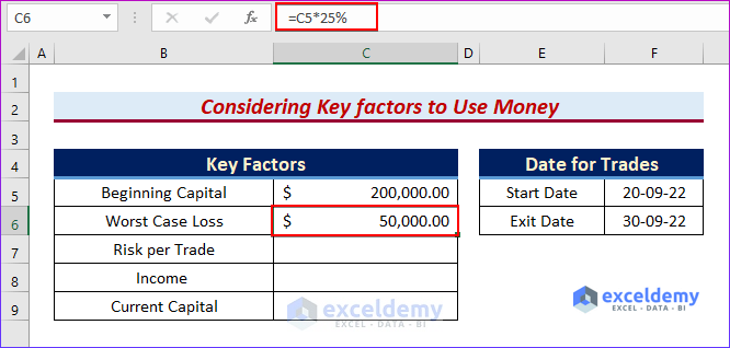
- Then, we keep our risk to 1%. This risk should be between 0.5% and 2%. If you take less than 0.5%, then your risk will be too low.
- So,write down this formula in cell C7.
=C5*1%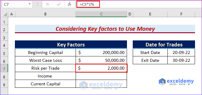
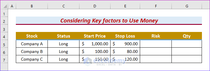
- Firstly, type the following fields:
- Stock → List the company you want to buy or sell.
- Status → Short or Long.
- Start Price → The price of the stock on the starting date.
- Stop Loss → To limit your loss.
- Risk → The difference between the “Start Price” and the “Stop Loss”.
- Qty → We will calculate this from these values and the risks from the first step.
- Secondly, write down all the details of the probable trades.
- Now, our values are higher in the Start Price column, if yours are not, then you can use this formula to get positive values.
- Thirdly, type the following formula in cell F5.
=ABS(D5-E5)- Then, press ENTER.
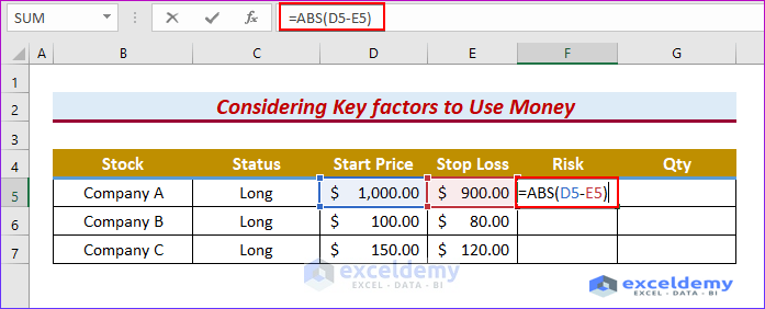
- So, you will see the Risk for the company A stocks in cell F5.
- Then, use the Fill Handle tool and drag it down from the F5 cell to the F7 cell.
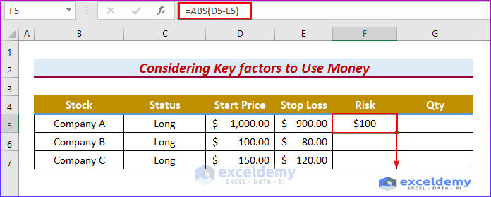
- Finally, you will get all the risks here in the below image.

Step 2: Calculating Trade Quantity Estimation
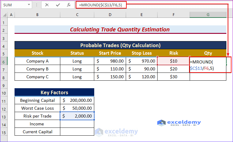
In this section, we will determine trade quantity estimation by using the MROUND function.
- So, we will find the quantity (Qty) of the trades for each company’s stocks.
- Then, type this formula into cell G6.
=MROUND($C$13/F6,5)- This formula divides the “Risk per Trade” amount by the “Risk of each company’s stock”. Then it rounds up or down to the nearest multiple of 5.
- Then, press ENTER.
- After that, you will see the estimated quantity for company A.
- Then, use the Fill Handle tool and drag it down from the G6 cell to the G8 cell.
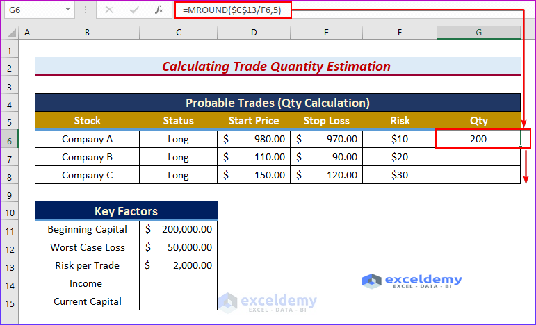
- Finally, you will get all the quantity for all the three companies.

Step 3: Inserting Transactions of Actual Trades
In this third step, we will add the values from a real trade to our money management Excel sheet. Moreover, we will be using the IF function to calculate profit or loss from the trades.
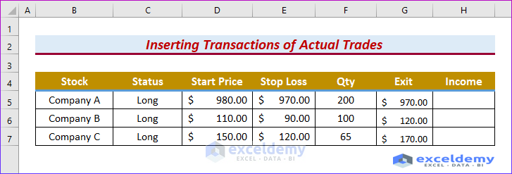
- First, type the following data into the sheet:
- Stock → List the company you want to buy or sell, taken from the last step.
- Status → Short or Long, taken from the last step.
- Start Price → The price of the stock on the starting date, taken from step 2.
- Qty → obtained from step 2.
- Stop Loss → To limit your loss, obtained from the last step.
- Exit Price → The selling price of the stocks.
- Income → Profit or loss gained from selling the stocks, which we will calculate using a formula.
- Then, type in the relevant data.
- Afterward, type the following formula in cell H5.
=IF(C5="Long",G5*F5-D5*F5,(D5*F5-E5*F5))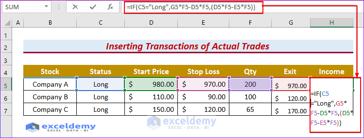
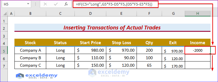
- The logical_test of this formula is C5 = ”Long”. If this is true, then the first part of the formula executes. Alternatively, the second part of the formula will be executed.
- Our formula reduces to → IF(TRUE,-2000,2000)
-
- Output: -2000.
-
- As this is true, the first part of the formula will be executed.
- Thus, we get the output.
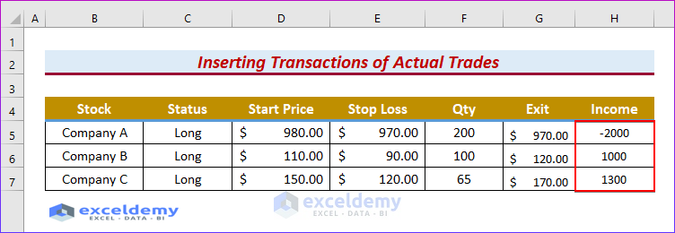
- Then, press ENTER and AutoFill the formula into the rest of the cells.
- Lastly, you will get all the output.
Step 4: Determining Total Income
Now, in the final step, we will be using the SUM function to get the total profit or loss for the trade, and we will fill in the last two cells from the first step.
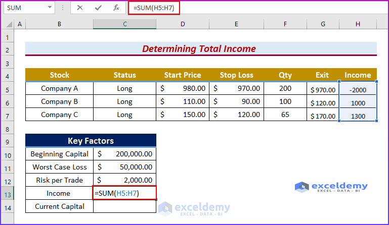
- Firstly, type the following formula in cell C13. This formula adds all the profit or loss from all the trades
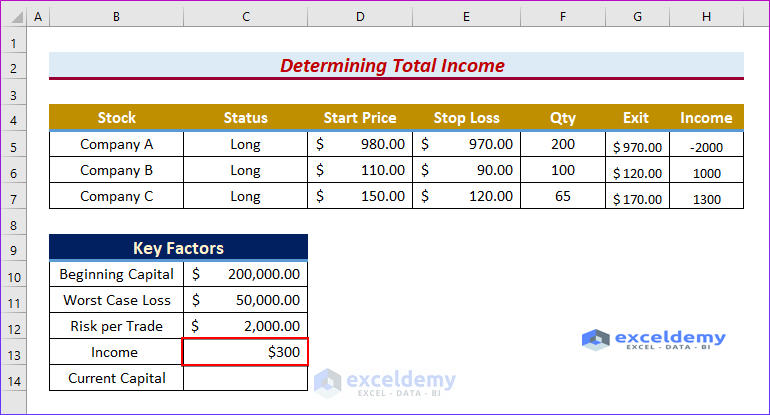
=SUM(H5:H7)- Then, press ENTER.
- So, you will get the income here in the below image.
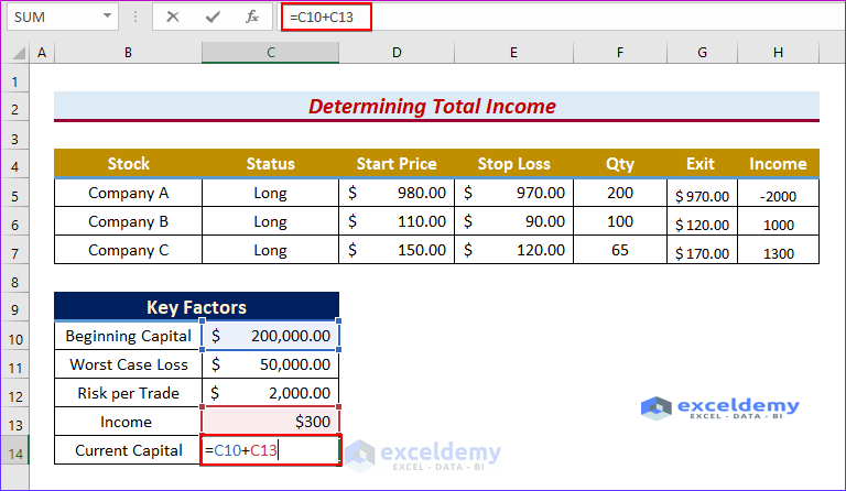
- After that, we will find the amount of “Current Capital” by typing this formula in cell C14.
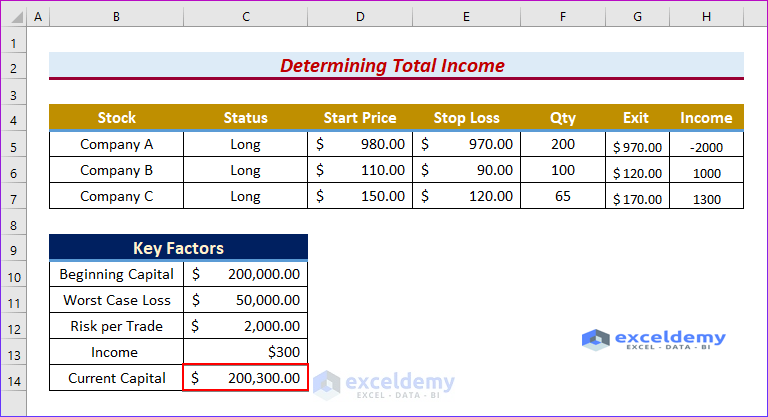
=C10+C13- Then, hit ENTER.
- As a result, you will find the current capital here.
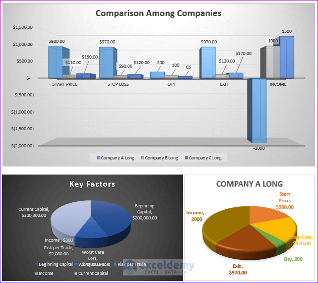
- Finally. this given image concludes the usages of money in Excel in terms of considering different factors such as individual income, total income. In the column chart, we have represented the individual income for the three companies A, B, and C respectively. Then, in the first pie chart, we have plotted the four key factors. And, in the rest pie chart, we have shown all the monetary details for a company (A).
Download Practice Workbook
You may download the following Excel workbook for better understanding and practice it yourself.
Conclusion
In this article, we’ve covered step-by-step procedures to use money in Excel.
We sincerely hope you enjoyed and learned a lot from this article. If you have any questions, comments, or recommendations, kindly leave them in the comment section below.
Get FREE Advanced Excel Exercises with Solutions!
