This is an overview:
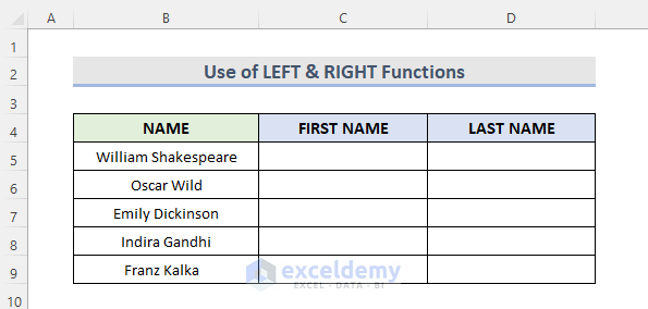
Method 1 – Using an Excel Formula with the LEFT & RIGHT Functions to Split a Cell
STEPS:
- Select C5.
- Enter the formula.
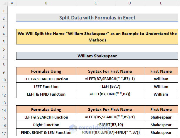
=LEFT(B5,SEARCH(" ",B5)-1)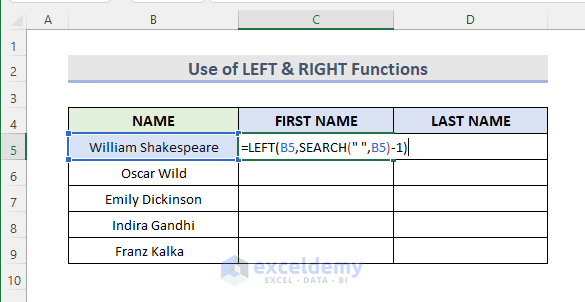
- Press Enter and use the Fill Handle to see the result.
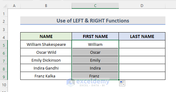
Formula Breakdown
SEARCH(” “,B5)
will search for the space and return the position of the space with the SEARCH function.
LEFT(B5,SEARCH(” “,B5)-1)
will extract all the characters on the left and return the value.
- Select D5 and enter the formula below.
=RIGHT(B5,LEN(B5)-SEARCH(" ",B5))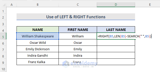
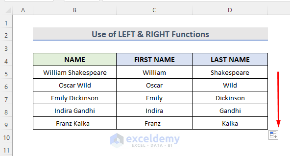
- Press Enter and use the Fill Handle to see the result.
Formula Breakdown
SEARCH(” “,B5)
returns the position of the space.
LEN(B5)
returns the total number of characters with the LEN function.
RIGHT(B5,LEN(B5)-SEARCH(” “,B5))
returns the last name value.
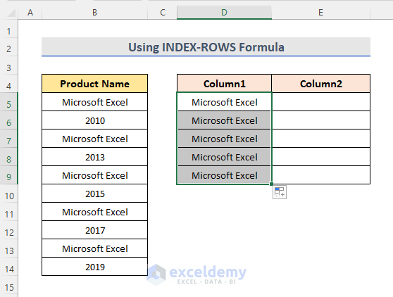
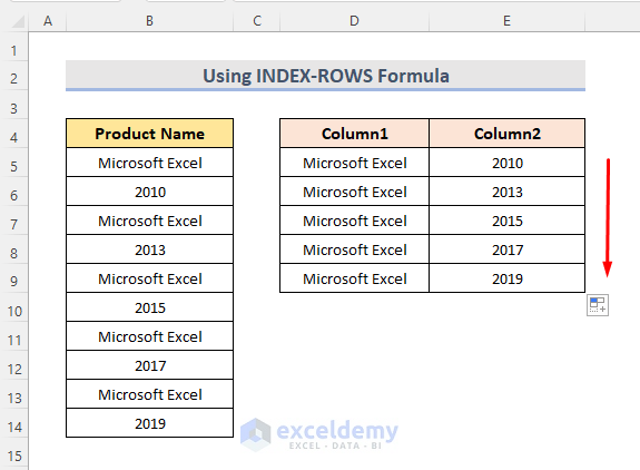
Method 2 – Using the INDEX-ROWS Formula to Split a Column into Multiple ones in Excel
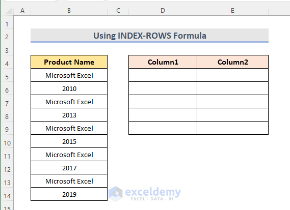
STEPS:
- Enter the formula in D5.
=INDEX($B$5:$B$14,ROWS(D$5:D5)*2-1)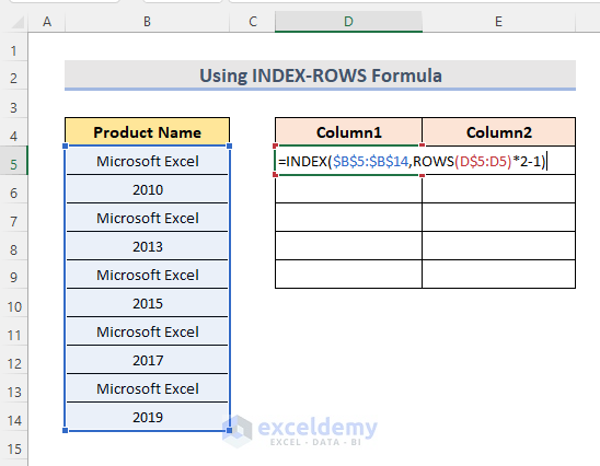
- Press Enter and use the Fill Handle to see the result.
Formula Breakdown
ROWS(D$5:D5)*2-1
returns the row number.
INDEX($B$5:$B$14,ROWS(D$5:D5)*2-1)
returns the value in $B$5:$B$14.
- Enter the formula in E5.
=INDEX($B$5:$B$14,ROWS(E$5:E5)*2)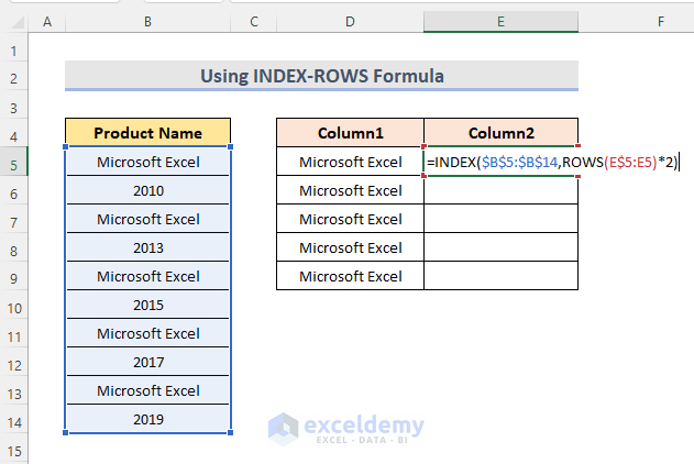
- Press Enter and use the Fill Handle to see the result.
Formula Breakdown
ROWS(E$5:E5)*2
returns the row number.
INDEX($B$5:$B$14,ROWS(E$5:E5)*2)
returns the value in $B$5:$B$14.
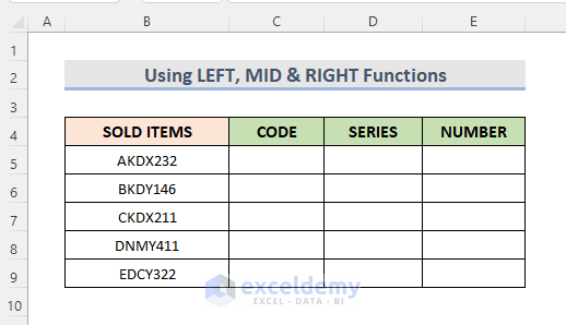
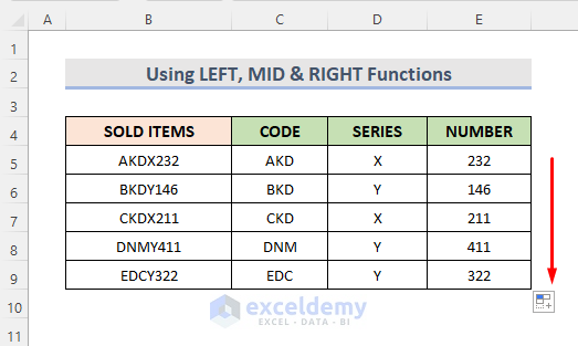
Method 3 – Using a Combination of the LEFT, MID & RIGHT Functions to Split a Text String
The dataset below showcases sold items in B4:E9. Split this column into three columns (CODE, SERIES, NUMBER).
STEPS:
- Select C5.
- Enter the formula below.
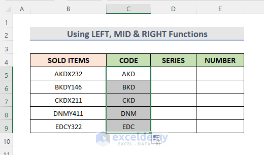
=LEFT(B5,3)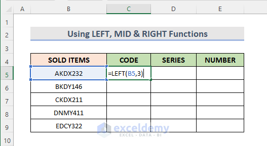
- Press Enter and use the Fill Handle to see the result.
- Enter the formula in D5.
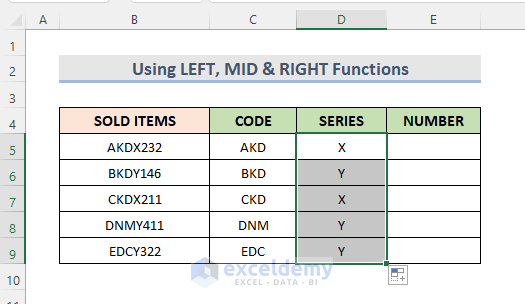
=MID(B5,4,1)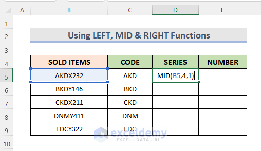
- Press Enter and use the Fill Handle to see the result.
- Select E5 and enter the formula.
=RIGHT(B5,3)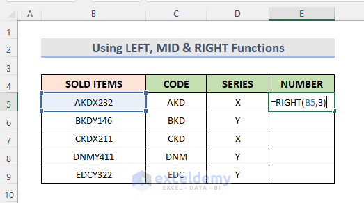
- Press Enter and use the Fill Handle to see the result.
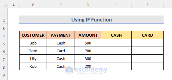
Method 4 – Using the IF Formula to Split
The dataset showcases customer payment history in B4:F8. Split the AMOUNT column into two columns (CASH & CARD).
- Select E5 and enter the formula.
=IF(C5="Cash",D5,"N/A")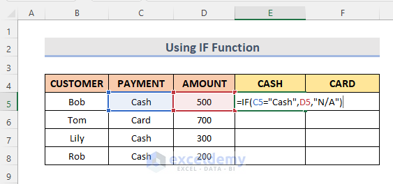
- Press Enter and use the Fill Handle to see the result.
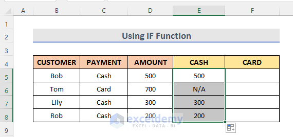
This formula will return the AMOUNT paid in Cash in E5. Otherwise, N/A.
- Select F5 and enter the formula below.
=IF(C5="Card",D5,"N/A")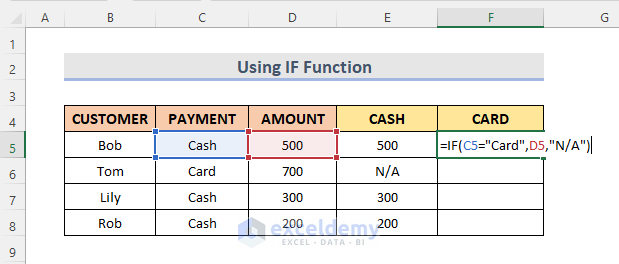
- Press Enter and use the Fill Handle to see the result.
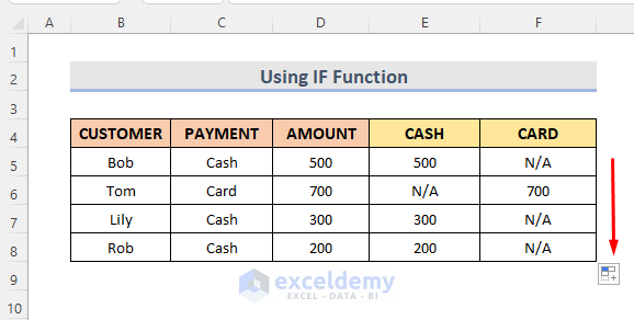
This formula will return the AMOUNT paid in Card in F5. Otherwise, N/A.
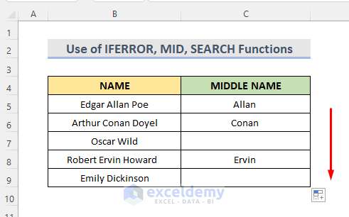
Method 5 – Combination of the IFERROR, MID and SEARCH Functions to Split the Middle Word
This is the sample dataset.
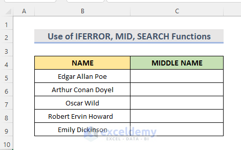
STEPS:
- Select D5 and use the formula below.
=IFERROR(MID(B5,SEARCH(" ",B5)+1,SEARCH(" ",B5,SEARCH(" ",B5)+1)-SEARCH(" ",B5)),"")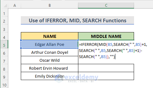
- Press Enter and use the Fill Handle to see the result.
Formula Breakdown
SEARCH(” “,B5)
returns the position of the space.
MID(B5,SEARCH(” “,B5)+1,SEARCH(” “,B5,SEARCH(” “,B5)+1)-SEARCH(” “,B5))
returns the middle word by using the position difference between the first and second spaces.
IFERROR(MID(B5,SEARCH(” “,B5)+1,SEARCH(” “,B5,SEARCH(” “,B5)+1)-SEARCH(” “,B5)),””)
returns a blank space if there is no middle word in the cell.
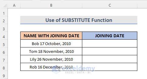
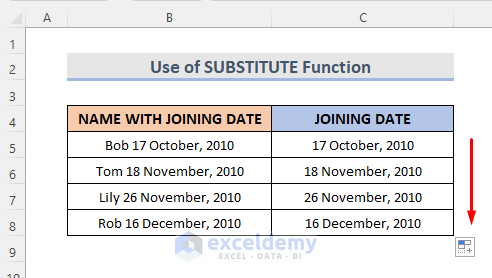
Method 6 – Using the SUBSTITUTE Function to Split a Date
This formula can only be used when there is a date at the end of the cell like in the dataset below (B4:C8).
STEPS:
- Enter the formula in C5.
=RIGHT(B5,LEN(B5)-FIND("~",SUBSTITUTE(B5," ","~",LEN(B5)-LEN(SUBSTITUTE(B5," ",""))-2)))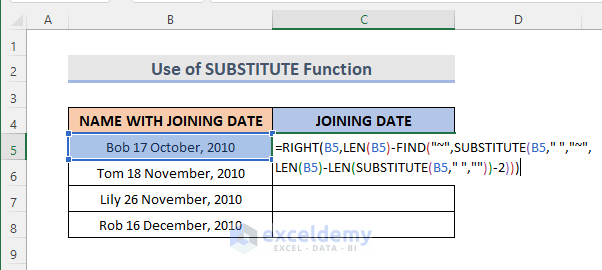
- Press Enter and use the Fill Handle to see the result.
Formula Breakdown
LEN(B5)
returns the length of the text string.
SUBSTITUTE(B5,” “,””)
replaces all the spaces in B5.
LEN(B5)-LEN(SUBSTITUTE(B5,” “,””))
subtracts the length without space from the total length.
SUBSTITUTE(B5,” “,”~”,LEN(B5)-LEN(SUBSTITUTE(B5,” “,””))-2)
places ‘~’ character between the name and the date.
FIND(“~”,SUBSTITUTE(B5,” “,”~”,LEN(B5)-LEN(SUBSTITUTE(B5,” “,””))-2))
finds the position of ‘~’ character, which is 4.
RIGHT(B5,LEN(B5)-FIND(“~”,SUBSTITUTE(B5,” “,”~”,LEN(B5)-LEN(SUBSTITUTE(B5,” “,””))-2)))
extracts the date from the text string.
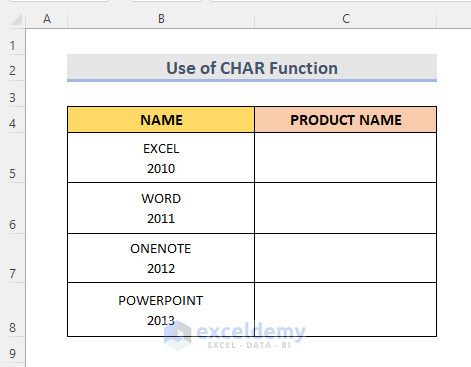
Method 7 – Using an Excel Formula to Split Text Using the CHAR Function
Extract the product name using. The ASCII code for the line is 10.
STEPS:
- Enter the formula in C5.
=LEFT(B5, SEARCH(CHAR(10),B5,1)-1)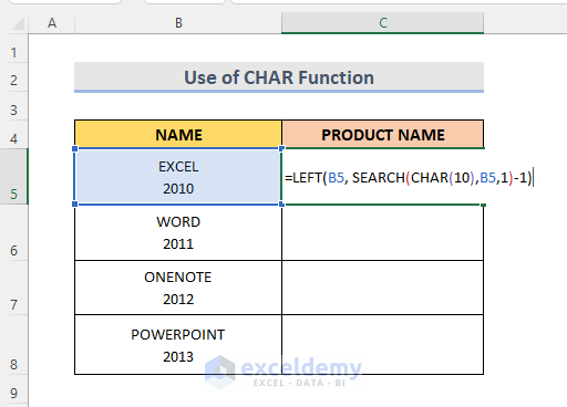
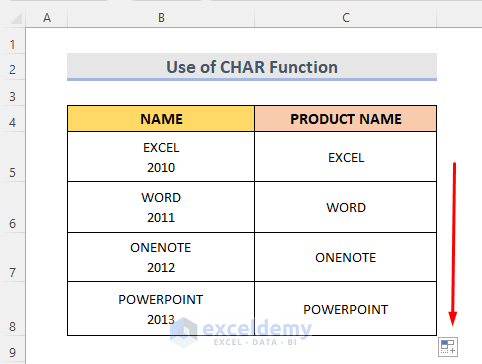
- Press Enter and use the Fill Handle to see the result.
Formula Breakdown
SEARCH(CHAR(10),B5,1)-1
searches for the position of the text string denoted by CHAR(10).
LEFT(B5, SEARCH(CHAR(10),B5,1)-1)
returns the leftmost value.
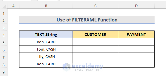
Method 8 – Using the FILTERXML Formula to Split text in Excel
Split customers’ names and payment methods.
STEPS:
- Select C5.
- Enter the formula.
=TRANSPOSE(FILTERXML("<t><s>"&SUBSTITUTE(B5,",","</s><s>")& "</s></t>","//s"))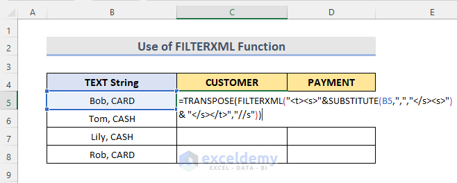
The sub-node is represented as s and the main-node is represented as t.
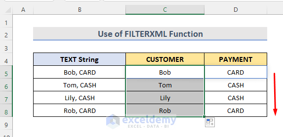
- Press Enter and use the Fill Handle to see the result.
Formula Breakdown
FILTERXML(“<t><s>”&SUBSTITUTE(B5,”,”,”</s><s>”)& “</s></t>”,”//s”)
turns the text strings into XML strings by changing the delimiter characters into XML tags.
TRANSPOSE(FILTERXML(“<t><s>”&SUBSTITUTE(B5,”,”,”</s><s>”)& “</s></t>”,”//s”))
The TRANSPOSE function returns the output horizontally instead of vertically.
Practice Workbook
Download the following workbook and exercise.
<< Go Back to Split in Excel | Learn Excel

