How to Split a Single Cell in Half in Excel

Excel has a lot of features that are meant for performing enormous operations and formatting. You may need to add two different types of headings in a single cell and for performing this task smartly, firstly you need to split a single cell in half. Then you can easily add one text to a split cell and another text to the other half.

If you are looking for the process of splitting a single cell in half, then you’re in the right place. This is the best-researched guide on the above topics.

Here, I will show you how to split a single cell in half in Excel.

In this section, you will find 2 methods to split a single cell in half in an Excel workbook. The processes will be applicable in any version of Excel from 2016 to 365. Here, I will demonstrate them with proper illustrations. Let’s check them now!

1. Splitting a Single Cell in Half in Excel Diagonally

In this section, I’ll show you the way to split a cell in half diagonally. This is the best method to split a cell in half (diagonally). Why? See the GIF image (below).

You see that whatever change I make with the cell; the format is not changing. That is what you want, right?

Let me show you how you can split a cell in that way. It is very easy.

1.1. Splitting Diagonally Down

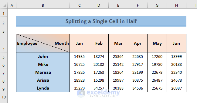
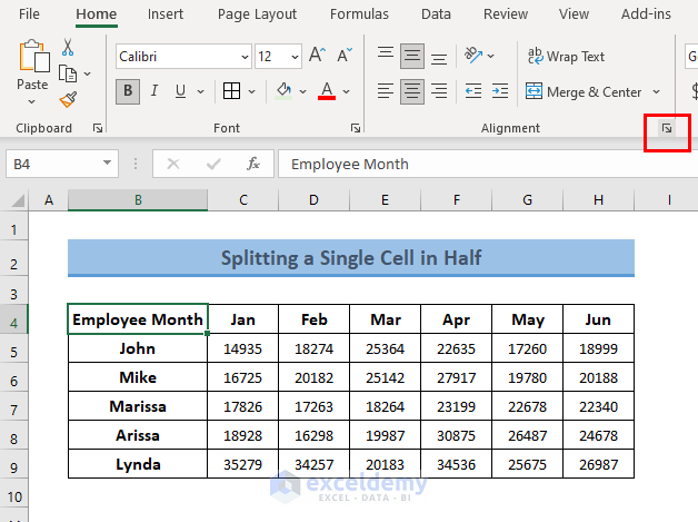
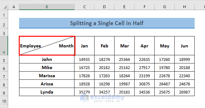
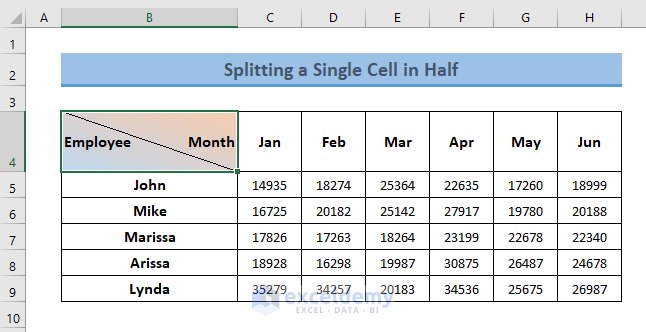
Let’s say, we have a dataset of some employees of an organization and their monthly sales (in USD) till half of the running year.

At the intersection of the row describing month and the column describing employee name, I have put two texts (i.e. Employee & Month). It looks so unprofessional if you put two types of texts in a single cell without splitting the cell. We want to split this cell into two so that one part contains the text “Employee” and another part takes “Month“. In order to serve this purpose, proceed with the following steps.

Steps:

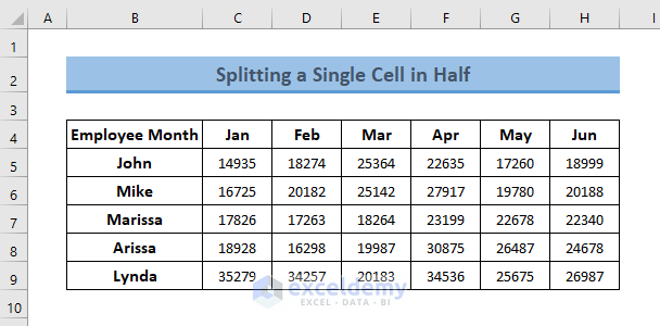
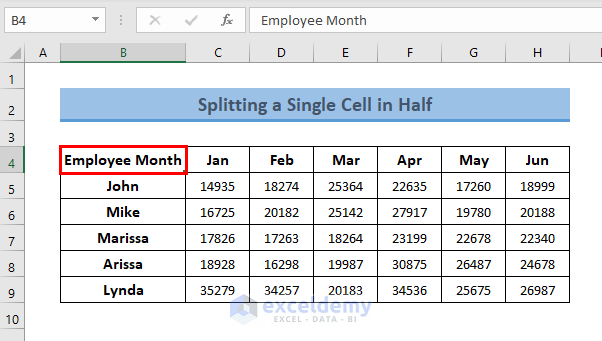
Select the cell that you want to split in half. And type your two words with space between them and press ENTER. In my case, I have typed Employee and Month in cell B4.

Now, go to the Home tab> click on the small arrow on the bottom-right corner of the Alignment group of commands.

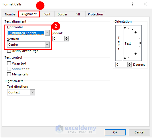
After that, open the Format Cells dialog box and go to the Alignment tab. The keyboard shortcut to open this dialog box is: CTRL + 1
In this dialog box, select the Distributed (Indent) option from the Horizontal menu and the Center option from the Vertical menu.

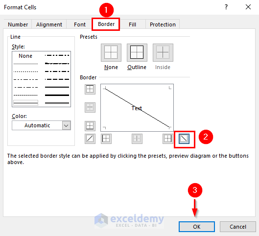
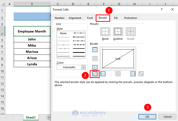
Now open the Border tab and select the diagonal down border (image below). You can choose also Border Line Style and Border Color from this window.
Finally, click on the OK button.

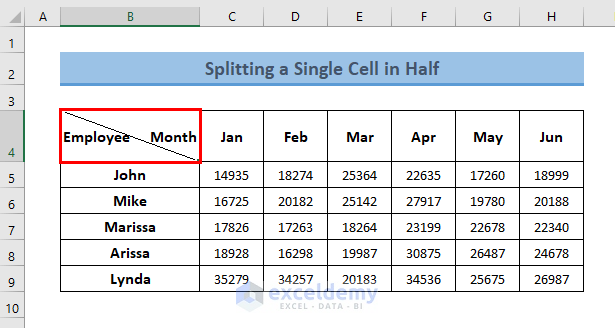
And you are done. Here is the output.

1.2. Splitting Diagonally Up

For the same set of data, if you want to split a cell in a diagonally up way, change the alignment just like you did for diagonally down but here, choose this border option from the Border tab.

And here is your result.

1.3. Splitting Cell Diagonally Using Objects

This is another method of splitting a cell in half in Excel. We shall use the Right Triangle Object to split a cell in half in this way.

Let’s start the process!

Steps:

Select a cell that you want to split and input one word (Employee) and make it Top Align.
Open the Insert tab -> Illustrations group of commands -> Click on the Shapes drop-down -> And select the Right Triangle from the Basic Shapes
Press and hold the Alt key and place the Right Triangle into the cell.
Then Flip the triangle horizontally and input the second word (Month).

The following GIF represents all the steps described above.

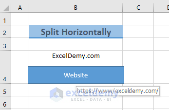
2. Splitting Single Excel Cell in Half Horizontally

Using the above method (Using Objects), you can also split a cell in half horizontally.

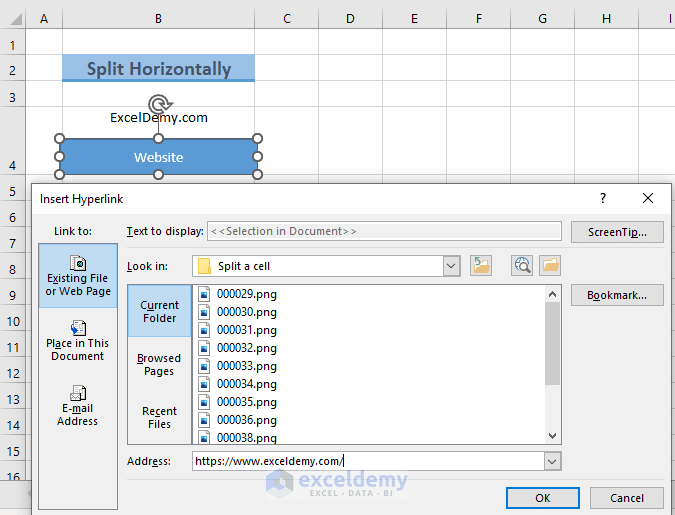
See the image below. I have used the Rectangle to draw the object into the cell. And then I have input a link to the object.

Here is the final output.

Add Two Background Colors to a Split Cell in Half in Excel

Let me show you how to split a cell diagonally with two background colors.

Steps:

Select the cell (already split in half)
Open the Format Cells dialog box
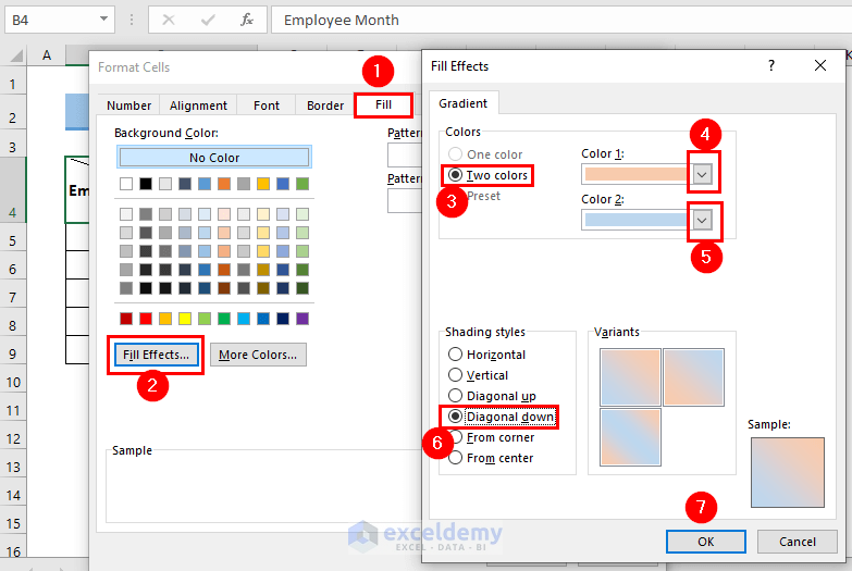
Open the Fill tab in the Format Cells dialog box
Click on the Fill Effects… command
Fill Effects dialog box will appear
In the Fill Effects dialog box, make sure that Two colors are selected in the Color option> choose a color for Color 1 open and choose another color for Color 2 field.
Select the Diagonal down from Shading styles
And finally, click on the OK button (two times)

You’re done. Here is the output.

Conclusion

So, these are my ways to split a cell in half in Excel. I showed both ways: diagonally and horizontally. Do you know a better way? Let me know in the comment box. Hope you like this blog post. Thanks for being with us!