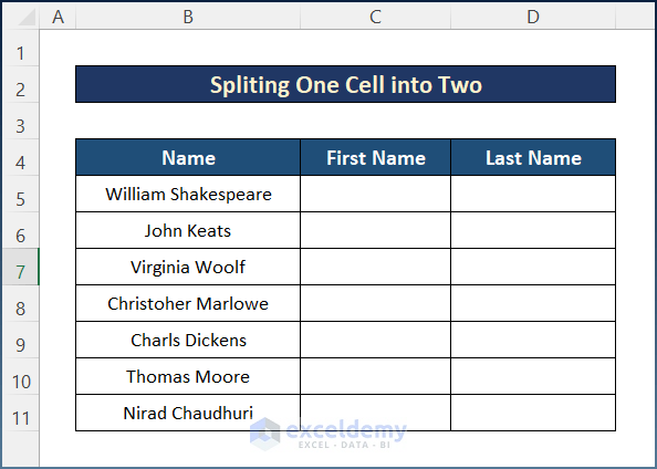
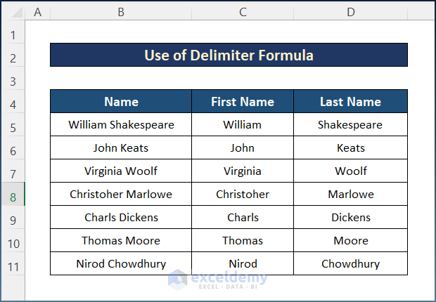
We have a dataset where column B consists of full names. We have to split the cells of column B into two columns, e.g., first name and last name.
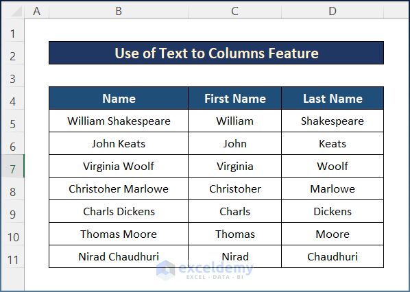
Method 1 – Split One Cell into Two Using the Text to Columns Feature
Steps:
- Select the whole dataset e.g. B4:B11.
- Pick the Text to Columns option from the Data tab.
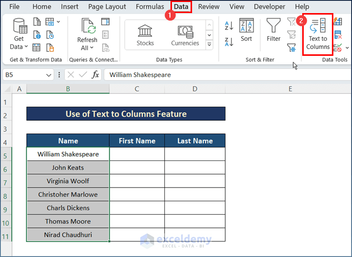
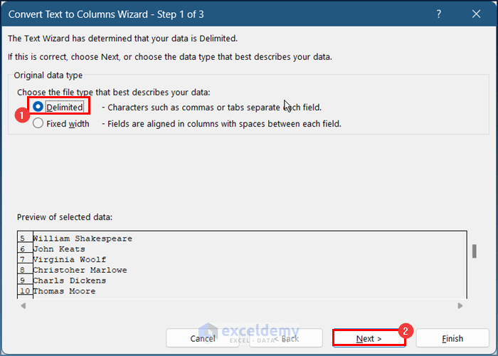
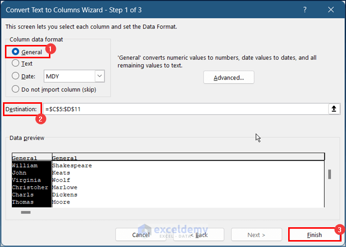
- The Text to Columns Wizard will appear.
- Choose the Delimited option and press Next.
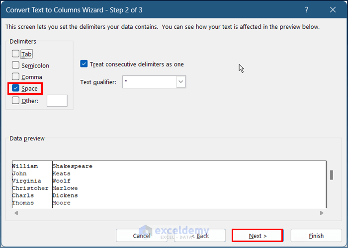
- Select the Space option and press Next.
- Select the Text option from the Column Data Format and adjust your Destination if necessary.
- Press Finish.
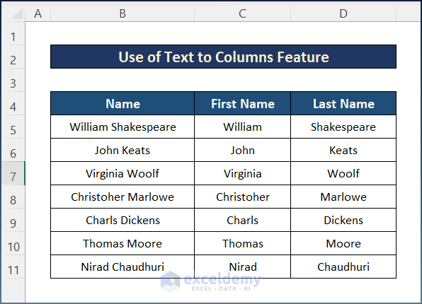
- You will get your final result.
Method 2 – Apply Flash Fill in Excel to Separate Cells
Steps:
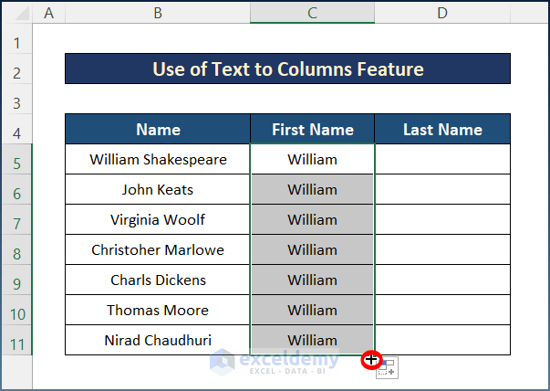
- Select a blank cell C5.
- Type in the first name William from the B5 cell in the selected cell C5.
- Use the AutoFill tool for the entire column.
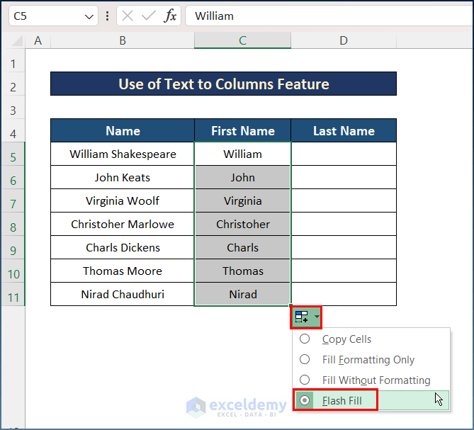
- Select the Flash Fill option to get your desired output.
- You can get the same output for the last names by repeating the process for the next column.
Read More: How to Split a Cell into Two Rows in Excel
Method 3 – Insert Formulas for Splitting One Cell into Two in Excel
Case 1 – Use a Delimiter
Our dataset uses the space as the delimiter, so we’ll use functions to detect its location and extract the text around it.
Steps:
- Select cell C5 and insert the following formula.
=LEFT(B5,FIND(" ",B5)-1)
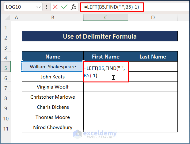
How Does the Formula Work?
- FIND(” “,B5): The FIND function looks for the space character (“ “) in Cell B5 and returns the position of that character which is ‘8’.
- FIND(” “,B5)-1: After subtracting 1 from the previous result, the new return value here is ‘7’.
- LEFT(B5,FIND(” “,B5)-1): Finally, the LEFT function extracts the 1st 6 characters from the text in Cell B5, which is ‘William’.
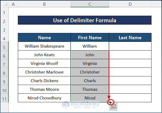
- Press the Enter key and use the AutoFill tool to the entire column.
- Use the following formula in cell D5.
=RIGHT(B5,LEN(B5)-FIND(" ",B5))
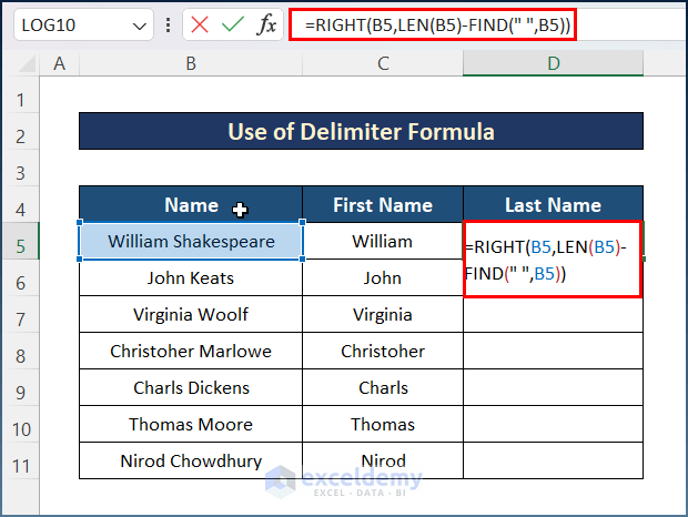
How Does the Formula Work?
- LEN(B5): The LEN function counts the number of total characters found in cell B5 and thereby returns ‘18’.
- FIND(” “,B5): The FIND function here again looks for the space character in cell B5 and returns the position which is ‘7’.
- LEN(B5)-FIND(” “,B5): This part of the entire formula returns ‘11’ which is the subtraction between the previous two outputs.
- RIGHT(B5,LEN(B5)-FIND(” “,B5)): Finally, the RIGHT function pulls out the last 11 characters from the text in Cell B5 and that is ‘Shakespeare’.
- Use the AutoFill tool to get the final output.
Read More: How to Split a Single Cell in Half in Excel
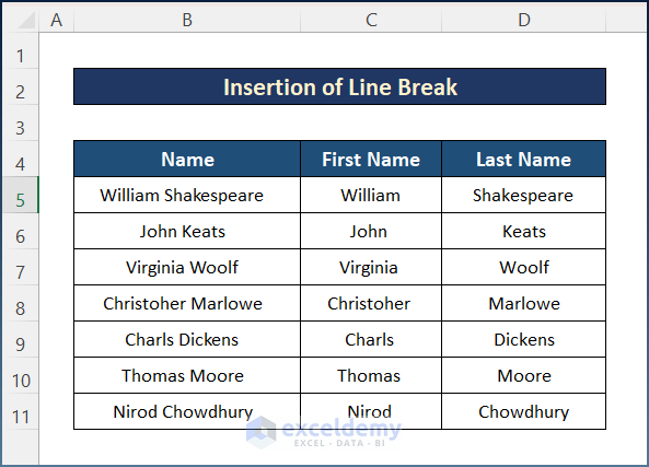
Case 2 – Insert Line Break
Steps:
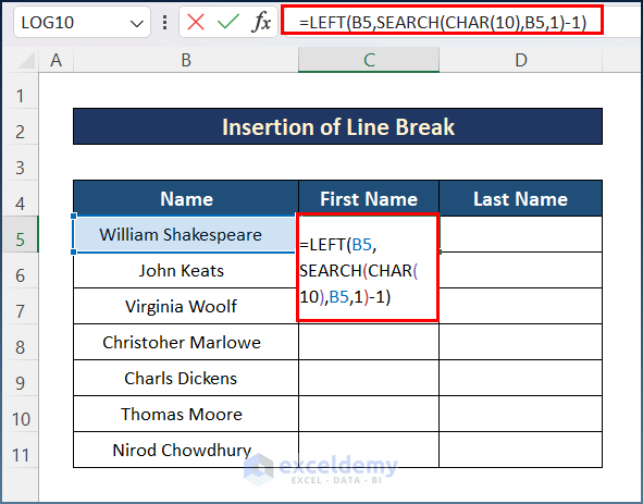
- Insert the following formula in cell C5.
=LEFT(B5,SEARCH(CHAR(10),B5,1)-1)
How Does the Formula Work?
- =SEARCH(CHAR(10),B5,1): This looks for the space character (“ “) in cell B5 and returns ‘9’.
- =LEFT(B5,SEARCH(CHAR(10),B5,1)-1): Finally, the LEFT function extracts the initial characters from the text in cell B5 which is ‘William’.
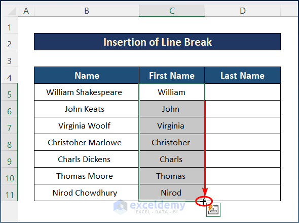
- Hit the Enter key and use the AutoFill tool to the whole column.
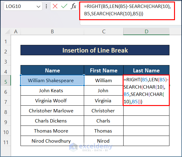
- Insert the formula below in cell D5.
=RIGHT(B5,LEN(B5)-SEARCH(CHAR(10),B5,SEARCH(CHAR(10),B5)))
How Does the Formula Work?
- =SEARCH(CHAR(10),B5): This looks for the space character (“ “) in Cell B5 and returns ‘9’.
- SEARCH(CHAR(10),B5,SEARCH(CHAR(10),B5)): also returns ‘9’.
- =RIGHT(B5,LEN(B5)-SEARCH(CHAR(10),B5,SEARCH(CHAR(10),B5))the ): Finally, the RIGHT function extracts the last characters from the text in cell B5 which is ‘Shakespeare’.
- Press the Enter key and use the AutoFill tool to get the final output.
Read More: Excel Formula to Split String by Comma
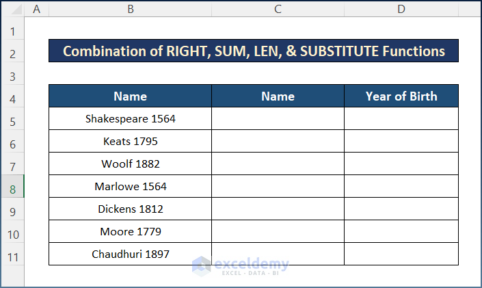
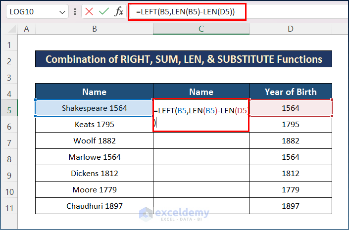
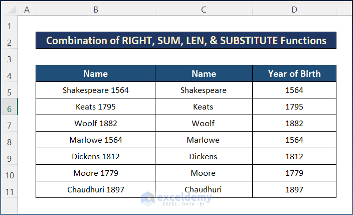
Method 4 – Combine RIGHT, SUM, LEN, and SUBSTITUTE Functions to Split Cells
We changed the dataset slightly to include a mix of names and numbers (the year of birth) in the order “Name DoB.”
Steps:
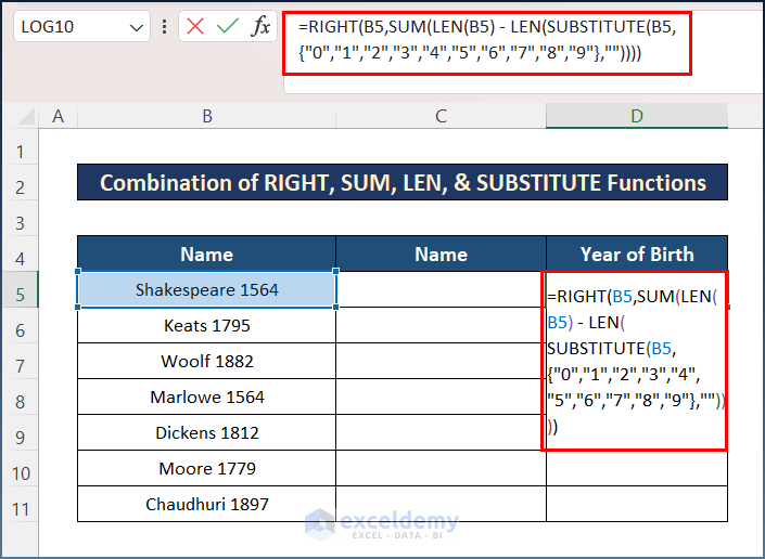
- Select cell D5 and insert the following formula.
=RIGHT(B5,SUM(LEN(B5) - LEN(SUBSTITUTE(B5,{"0","1","2","3","4","5","6","7","8","9"},""))))
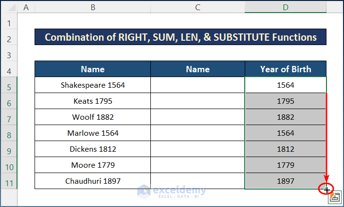
- Press Enter and apply the AutoFill tool.
- Use the following formula in cell C5.
=LEFT(B5,LEN(B5)-LEN(D5))
- Hit the Enter key and apply the AutoFill tool to get the desired output.
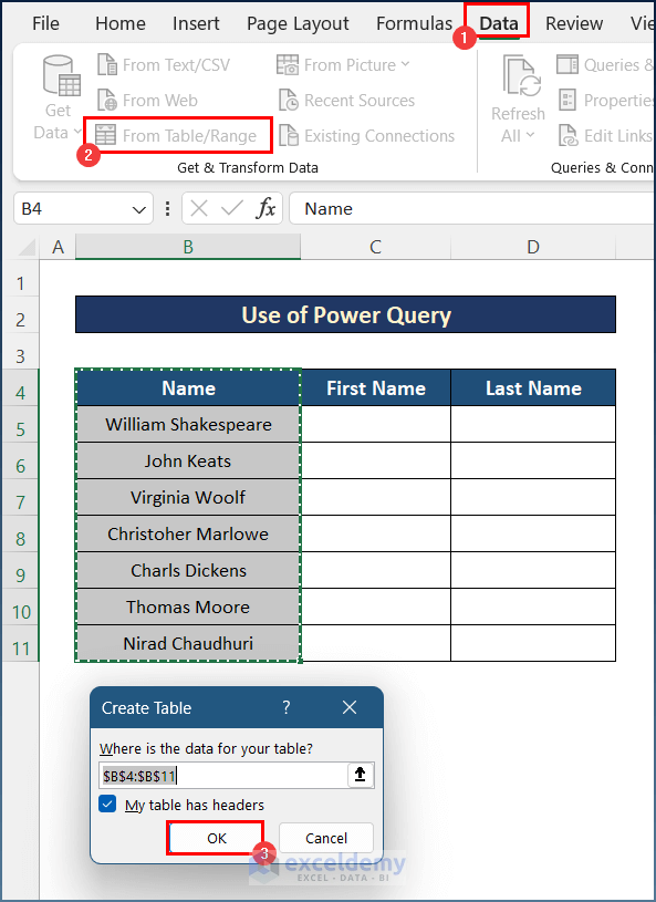
Method 5 – Break One Cell into Two Through Excel Power Query
Steps:
- Select the entire column, including the header.
- Go to the Data tab and click on From Table/Range.
- Press OK.
- You’ll get the Power Query Editor,
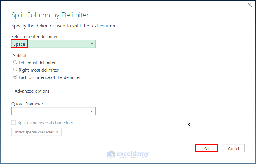
- Go to Home, select Split Column, and choose By Delimiter.
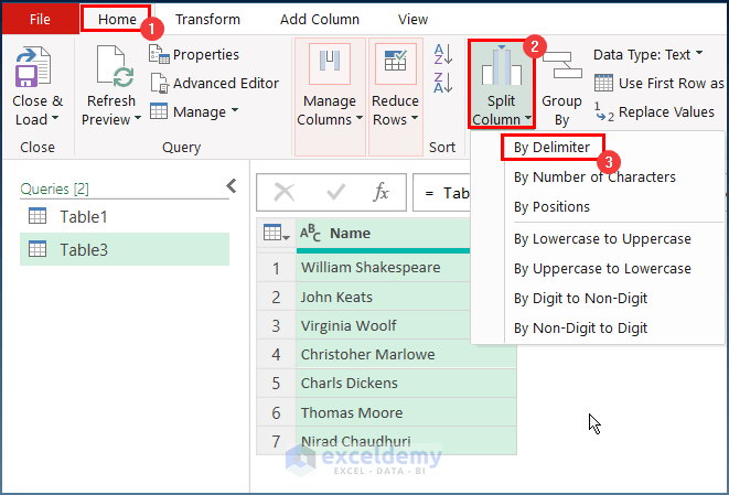
- Select Space as your delimiter and press OK.
- Click on Close & Load, then on Close & Load To.
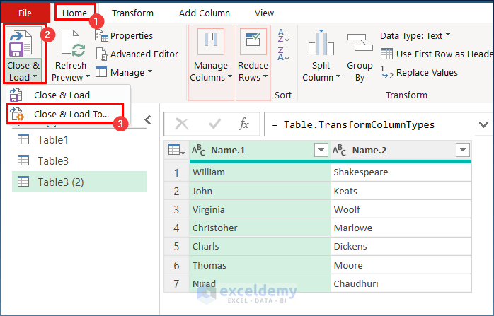
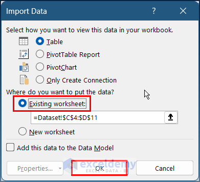
- Choose your destination in the Import Data dialog box and press OK.
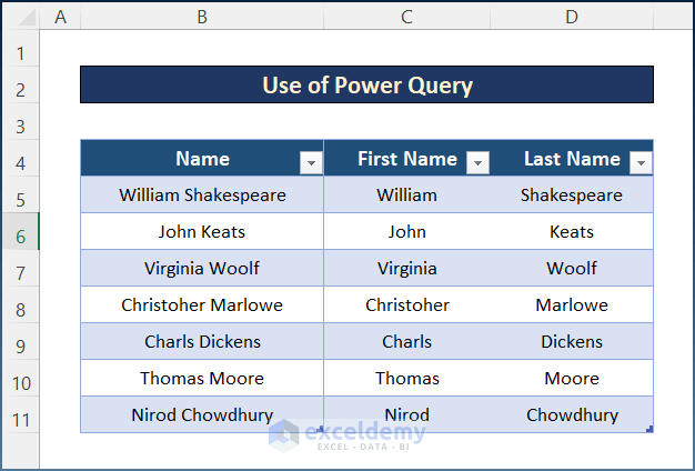
- Here’s the output.
Read More: How to Split Cell by Delimiter Using Excel Formula
Download the Practice Workbook
Get FREE Advanced Excel Exercises with Solutions!

split 1000 – 1200 in a cell into 2 cells
eg.
1000 1200 into 2 cells
Hello Ng Chin Hwa,
You can split “1000 – 1200” into two cells using Excel’s Text to Columns feature:
1. Select the cell with “1000 – 1200”.
2. Go to the Data tab → Click Text to Columns.
3. Choose Delimited → Click Next.
4. Check the Other box and enter the dash (–) as the delimiter.
5. Click Finish.
Now “1000” will go into one cell and “1200” into the next!
Regards
ExcelDemy