How to Split a Cell into Two Rows in Excel (3 Easy Ways)

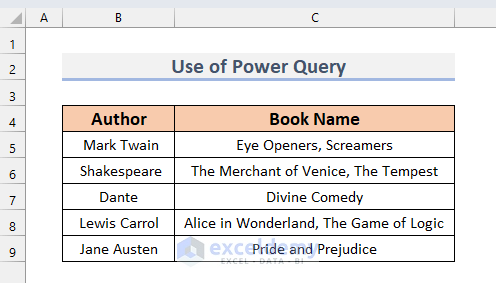
Here’s an overview of splitting a cell into two rows in Excel.

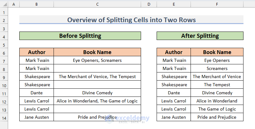
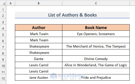
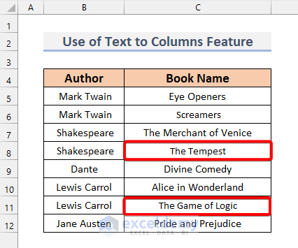
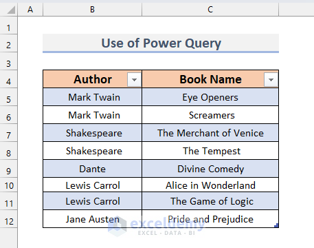
We’ll use dataset with two columns: Author and Book Name. There are some cells where multiple book names are in one cell (C5, C7, C10). We will split the names of books in cells C5, C7, and C10 into two rows (C5:C6, C7:C8, and C10: C11 respectively). Let’s explore the methods one by one to accomplish our goal.

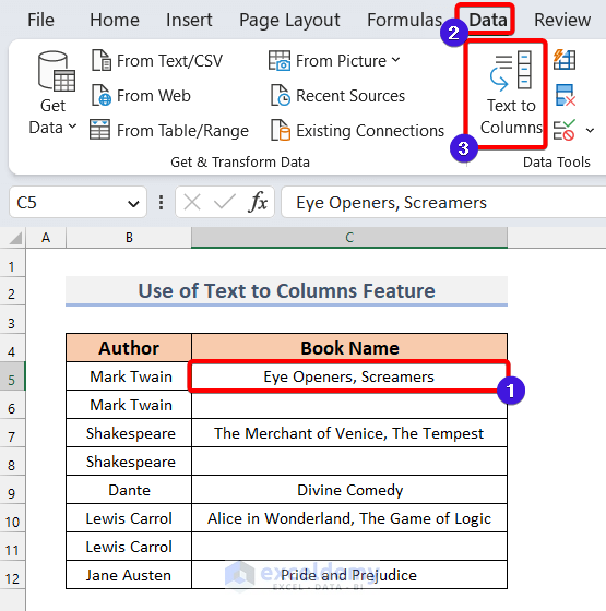
Method 1 – Using the Text to Columns Feature to Split a Cell into Two Rows in Excel

Steps:

• Select the cell that you want to split. We selected cell C5.
• Open the Data tab.
• From Data Tools, select the Text to Columns option.

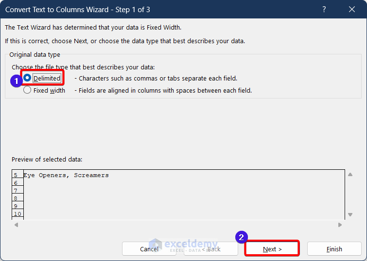
• A dialog box named Convert Text to Columns Wizard will pop up.
• Select the file type Delimited and click Next.

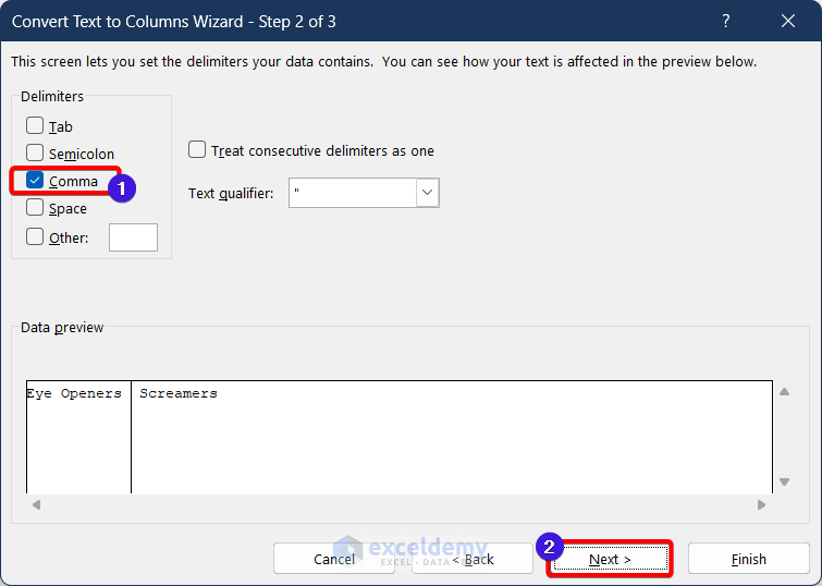
• In step 2, select the Delimiters by which your text will be separated. In our case, the names are separated by a comma (,), so we selected a comma (,).
• Click Next.

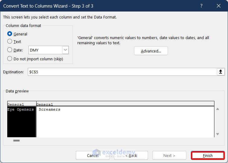
• In step 3, if you want to place the separated texts in a different location, you can choose a Destination. Otherwise, keep the field as it is.
• Click Finish.

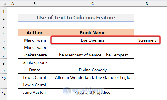
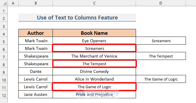
• You will see that the values are split into two columns (C5 and D5).

• To convert the split columns into rows, we can take two different approaches.

Read More: How to Split One Cell into Two in Excel

Option 1.1 – Using the Cut-Paste Option

Steps:

• Select cell D5.
• Press Ctrl + X.
• Go to cell D6.
• Press Ctrl + V.

• Repeat the entire process for cells C7 and C10 and obtain the desired result.

Read More: How to Split a Single Cell in Half in Excel

Option 1.2 – Using the TRANSPOSE Function

Steps:

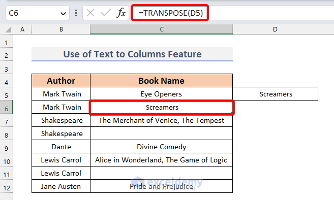
• Select the cell to place your value. We selected cell C6.
• Use the following formula in the selected cell or into the Formula Bar.

• Click Enter.

• Apply the same formula in cells C7 and C10.

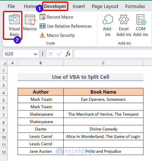
Method 2 – Using Excel VBA to Split a Cell into Two Rows

Steps:

• Open the Developer tab.
• Select Visual Basic.

• This will open a new window for Microsoft Visual Basic for Applications.
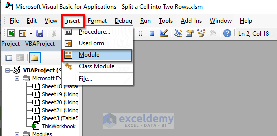
• Click on Insert and choose Module to open a new module.

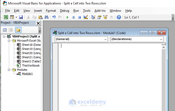
• A new Module will open.

• Insert the following code in the Module.

Sub Split_Cell_into_Rows()
Dim rng As Range
Dim InputRng As Range, OutputRng As Range
ExcelTitleId = "Split Cell into Rows"
Set InputRng = Application.Selection.Range("A1")
Set InputRng = Application.InputBox("Select the cell to be split(single cell) :", ExcelTitleId, InputRng.Address, Type:=8)
Set OutputRng = Application.InputBox("Select the range of rows (a range):", ExcelTitleId, Type:=8)
Arr = VBA.Split(InputRng.Range("A1").Value, ",")
OutputRng.Resize(UBound(Arr) - LBound(Arr) + 1).Value = Application.Transpose(Arr)
End Sub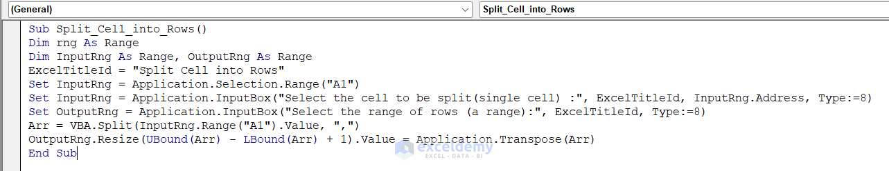

• Save the code and go back to the worksheet.
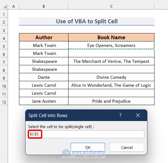
• Select the cell that you want to split into rows. We selected cell C5.
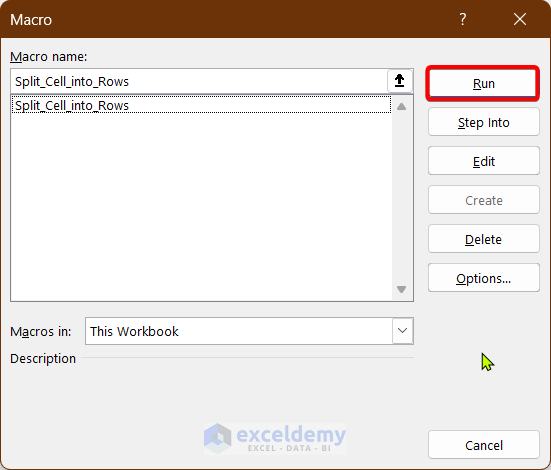
• Open the Macro dialog box with Alt + F8.
• Select the Macro to Run.

• A dialog box will pop up named Split Cell into Rows. Select the cell first or range.

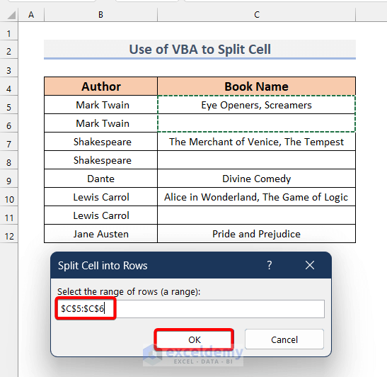
• Select the range where you want to place the split values of a cell. We selected the range C5:C6.

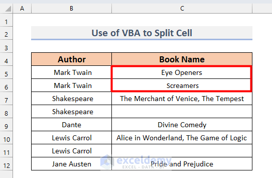
• You will see the selected cell’s value is split into two rows.

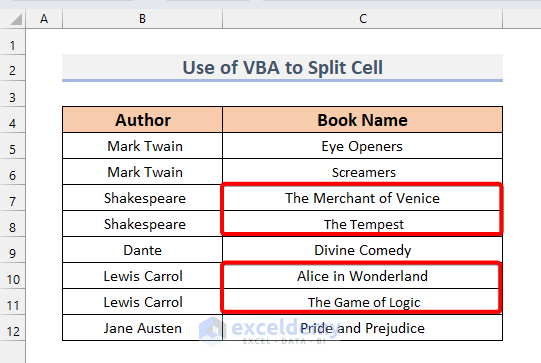
• We can follow the same process to split cells C7 and C10 into two rows C7:C8, and C10: C11

Read More: How to Split Cell by Delimiter Using Excel Formula

Method 3 – Using Power Query to Split a Cell into Two Rows in Excel

We removed the rows with blank cells, so we need to add them back when splitting.

Steps:

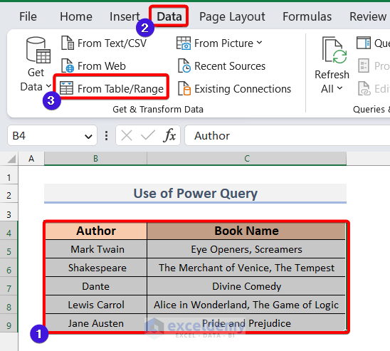
• Select the entire dataset.
• Open the Data tab.
• Select the From Table/Range option from the ribbon.

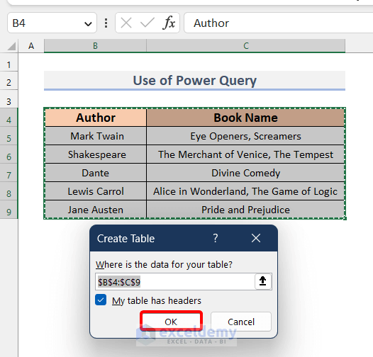
• A dialog box will pop up. Select My table has headers.
• Click OK.

• The Power Query Editor window will pop up.

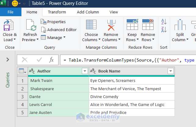
• Select any cell that you want to split into two rows.
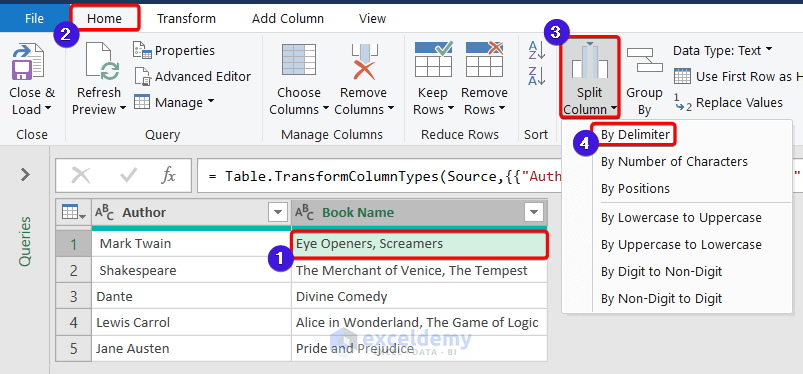
• Go to the Home tab.
• Click on Split Column and select By Delimiter.

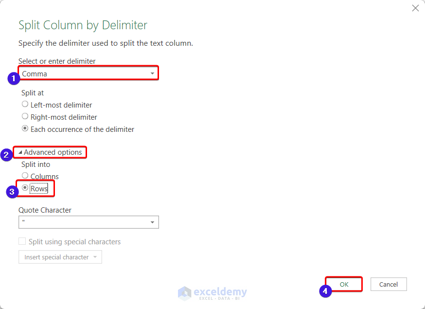
• A dialog box will pop up. Select the Delimiter comma(,), then click on the Advanced Options.
• Select Rows.
• Click OK.

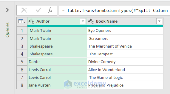
• You will see that all the cells that contain a delimiter(comma) have been split into multiple rows. The adjacent cells in the left column were also duplicated.

• Click the Close & Load option from the ribbon to load the data in another sheet in the workbook.

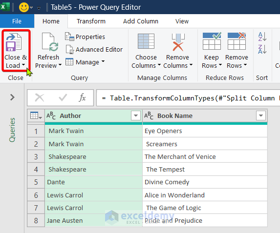
• The table will be loaded into a separate sheet.
• After some formatting, the final result will be like this below.

Read More: Excel Formula to Split String by Comma

Download the Practice Workbook