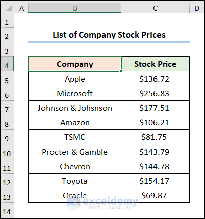
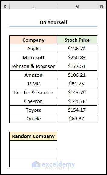
How to Randomize a List Without Duplicates in Excel

The dataset showcases a List of Stock Prices.

Method 1 – Using the INDEX, SORTBY, and SEQUENCE Functions

Combine the INDEX, SORTBY, RANDARRAY, ROWS, and SEQUENCE functions to select 3 random “Companies” .

Steps:

Select B16 and enter the formula below.

=INDEX(SORTBY(B5:B13, RANDARRAY(ROWS(B5:B13))), SEQUENCE(3))

B5:B13 refers to the “Company” names.

Formula Breakdown:

ROWS(B5:B13) → returns the total row number in the given range.
- Output → 9
RANDARRAY(ROWS(B4:B12)) → returns an array of random numbers, here, 9. The ROWS(B4:B12) is the optional rows argument.
- Output → {0.278134626212438;0.148720604883087;0.355282358043423;0.036883208689009;0.832535669722357;0.927487306458828;0.223257349246205;0.241979490824856;0.100170115552212}
SORTBY(B4:B12, RANDARRAY(ROWS(B4:B12))) → sorts a range or array based on the values in the corresponding range or arrays. Here, B4:B12 is the array argument and the RANDARRAY(ROWS(B4:B12)) is the by_array_1 argument.
- Output → {“Amazon”;”Microsoft”;”Johnson & Johnson”;”Procter & Gamble”;”Oracle”;”TSMC”;”Chevron”;”Apple”;”Toyota”}

SEQUENCE(3) → returns a sequence of numbers. Here, 3 is the rows argument.
- Output → {1;2;3}

=INDEX(SORTBY(B5:B13, RANDARRAY(ROWS(B5:B13))), SEQUENCE(3)) → returns a value at the intersection of a row and column in a given range. In this expression, SORTBY(B5:B13, RANDARRAY(ROWS(B5:B13))) is the array argument and SEQUENCE(3) is the row_num argument that indicates the row location.
- Output → {“Chevron”, “Procter & Gamble”, “Toyota”}

Note: This formula works for the Excel 365 and Excel 2021 versions, if you’re using an older version of Excel, apply the next method.

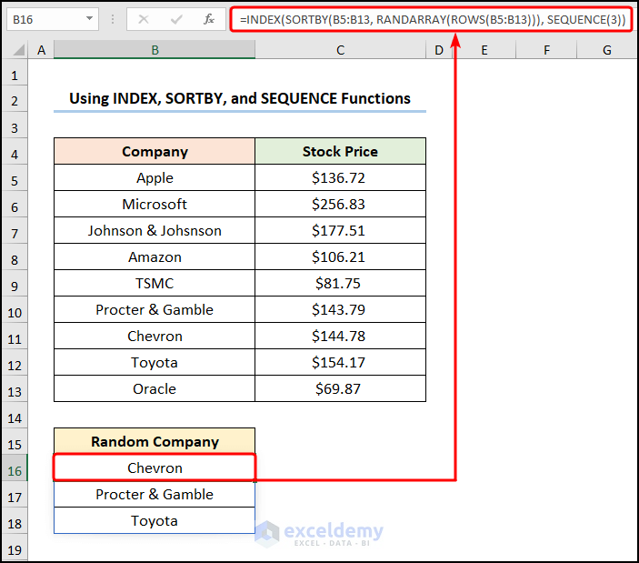
The result is a randomized list without duplicates.

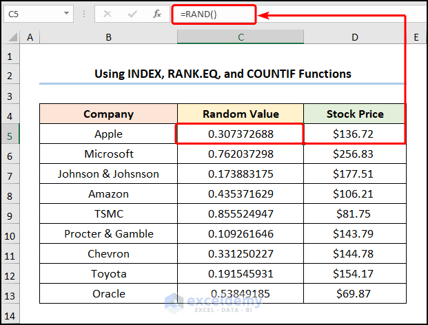
Method 2 – Utilizing the INDEX, RANK.EQ, and COUNTIF Functions

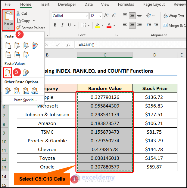
Combine the RAND, INDEX, RANK.EQ, and COUNTIF functions to obtain a randomized list of the “Company” names.

Steps:

Go to C5 >> use the RAND function to generate a random value >>Drag down the Fill Handle to see the result in the rest of the cells.

Select C5:C13 >> press CTRL + C to copy the values.

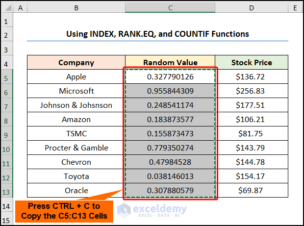
Choose C5:C13 >> click Paste >> select Paste Values.

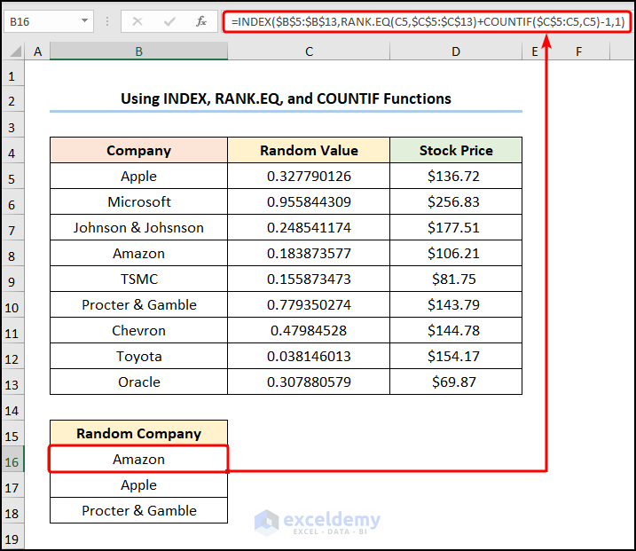
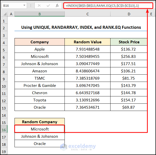
Go to B16 and enter the following formula.

=INDEX($B$5:$B$13,RANK.EQ(C5,$C$5:$C$13)+COUNTIF($C$5:C5,C5)-1,1)

B5:B13 and C5:C13 represent “Company” and “Random Values” . C5 cell points to the first “Random Value”.

Formula Breakdown:

RANK.EQ(C5,$C$5:$C$13) → returns the rank of a value in a list of numbers. C5 is the number argument and $C$5:$C$13 refers to the ref argument.
- Output → 9
COUNTIF($C$5:C5,C5) → counts the number of cells within a range that meet the given condition. $C$5:C5 represents the range argument that refers to the first “Random Value”. C5 indicates the criteria argument that returns the count of the matched value.
- Output → 1

INDEX($B$5:$B$13,RANK.EQ(C5,$C$5:$C$13)+COUNTIF($C$5:C5,C5)-1,1) → $B$5:$B$13 is the array argument: the “Company” name. RANK.EQ(C5,$C$5:$C$13)+COUNTIF($C$5:C5,C5)-1 is the row_num argument that indicates the row location. 1 is the optional column_num argument that points to the column location.
- Output → “Oracle”

Note: Use Absolute Cell Reference by pressing F4.

Method 3 – Using the RAND, INDEX, and RANK.EQ Functions

Use the RAND, INDEX, and RANK.EQ functions to get 3 random “Company” names.

Steps:

Follow the steps shown previously or the GIF to copy and paste values in the “Random Value” column.

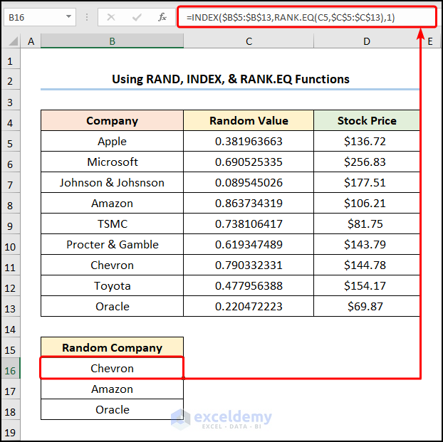
Select B16 >> enter the formula in the Formula Bar.

=INDEX($B$5:$B$13,RANK.EQ(C5,$C$5:$C$13),1)

B5:B13 and C5:C13 indicate “Company” and “Random Values” and C5 represents the initial “Random Value”.

Formula Breakdown:

RANK.EQ(C5,$C$5:$C$13) → C5 is the number argument and $C$5:$C$13 refers to the ref argument.
- Output → 7

INDEX($B$5:$B$13,RANK.EQ(C5,$C$5:$C$13),1) → $B$5:$B$13 is the array argument: the “Company” name. RANK.EQ(C5,$C$5:$C$13) is the row_num argument that indicates the row location. 1 is the optional column_num argument that points to the column location.
- Output → “Chevron”

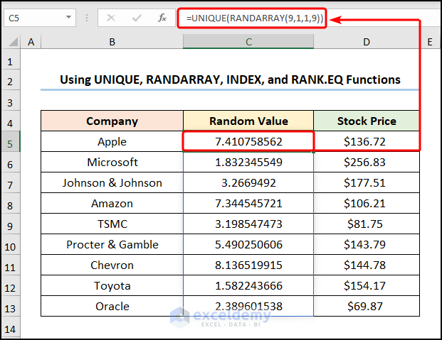
Method 4 – Applying the UNIQUE, RANDARRAY, INDEX, and RANK.EQ Functions

Apply the UNIQUE, RANDARRAY, INDEX, RANK.EQ functions to get a list of random values.

Steps:

Select C5 and enter the formula below.

=UNIQUE(RANDARRAY(9,1,1,9))

9 is the row number, 1 is the column number, 1 is the minimum number, and 9 is the maximum number. The UNIQUE function ensures the RANDARRAY function returns an array of unique numbers.

Note: To stop C5:C13 from changing, copy and paste the values only or follow the steps shown in the previous method.

Use the following equation in B16.

=INDEX($B$5:$B$13,RANK.EQ(C5,$C$5:$C$13),1)

B5:B13 and C5:C13 point to “Company” and “Random Values”.

How to Randomly Select from a List with No Duplicates in Excel

Get the “Company” names and their corresponding “Stock Prices” using the SORTBY, RANDARRAY, INDEX, SEQUENCE, and ROWS functions.

Steps:

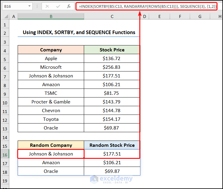
Enter the formula in B16.

=INDEX(SORTBY(B5:C13, RANDARRAY(ROWS(B5:C13))), SEQUENCE(3), {1,2})

Formula Breakdown:

ROWS(B5:C13) → 9
RANDARRAY(ROWS(B5:C13)) → ROWS(B5:C13) is the optional rows argument.
- Output → {0.0140698270891861;0.336601258084547;0.302828885068347;0.458536948594194;0.349731499694981;0.188127312170481;0.901260642146929;0.455208105393427;0.480186486777415}
SORTBY(B5:C13, RANDARRAY(ROWS(B5:C13))) → B5:C13 is the array argument and RANDARRAY(ROWS(B5:C13)) is the by_array_1 argument.
- Output → {“TSMC”,81.75;”Toyota”,154.17;”Amazon”,106.21;”Apple”,136.72;”Microsoft”,256.83;”Procter & Gamble”,143.79;”Johnson & Johnson”,177.51;”Chevron”,144.78;”Oracle”,69.87}

SEQUENCE(3) → 3 is the rows argument.
- Output → {1;2;3}

INDEX(SORTBY(B5:C13, RANDARRAY(ROWS(B5:C13))), SEQUENCE(3), {1,2}) → SORTBY(B5:C13, RANDARRAY(ROWS(B5:C13))) is the array argument and SEQUENCE(3) and {1,2} are the row_num and col_num arguments indicating the row and column locations.

How to Randomly Select with Criteria in Excel

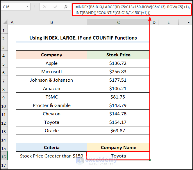
Use the INDEX, LARGE, IF, ROW, INT, RAND, and COUNTIF functions to calculate the “Company” with a “Stock Price” greater than “$150 USD”.

Steps:

Enter the formula in C16.

=INDEX(B5:B13,LARGE(IF(C5:C13>150,ROW(C5:C13)-ROW(C5)+1),INT(RAND()*COUNTIF(C5:C13,">150")+1)))

Formula Breakdown:

IF(C5:C13>150,ROW(C5:C13)-ROW(C5)+1) → checks whether a condition is met and returns one value if TRUE and another if FALSE. C5:C13>150 is the logical_test argument that compares the values in C5:C13 range with 150. If this value is greater than or equal to 150, the function returns ROW(C5:C13)-ROW(C5)+1) (value_if_true argument). Otherwise, it returns Blank (value_if_false argument).
- Output → {FALSE;2;3;FALSE;FALSE;FALSE;FALSE;8;FALSE}
COUNTIF(C5:C13,”>150″) → C5:C13 represents the range argument that refers to the Stock Prices, and “>150” indicates the criteria argument that returns the count of the matched value.
- Output → 3
INT(RAND()*COUNTIF(C5:C13,”>150″)+1) → rounds a number down to the nearest integer. RAND()*COUNTIF(C5:C13,”>150″)+1 is the number argument.
- 0.305982491187225 * 3 + 1 → 3
LARGE(IF(C5:C13>150,ROW(C5:C13)-ROW(C5)+1),INT(RAND()*COUNTIF(C5:C13,”>150″)+1))→ returns the k-th largest in a dataset. IF(C5:C13>150,ROW(C5:C13)-ROW(C5)+1) is the array argument and INT(RAND()*COUNTIF(C5:C13,”>150″)+1) is the k-th argument.
- Output → 8
INDEX(B5:B13,LARGE(IF(C5:C13>150,ROW(C5:C13)-ROW(C5)+1),INT(RAND()*COUNTIF(C5:C13,”>150″)+1))) → B5:B13 is the array argument: the “Company” name. LARGE(IF(C5:C13>150,ROW(C5:C13)-ROW(C5)+1),INT(RAND()*COUNTIF(C5:C13,”>150″)+1)) is the row_num argument that indicates the row location.
- Output → “Toyota”

Note: In older versions of Excel, press CTRL + SHIFT + ENTER to use an array formula.

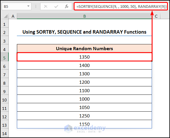
How to Create a Unique Random Number Generator in Excel

Use the SORTBY, SEQUENCE, and RANDARRAY functions.

Steps:

Enter the formula in B5.

=SORTBY(SEQUENCE(9, , 1000, 50), RANDARRAY(9))

Formula Breakdown:

SEQUENCE(9, , 1000, 50) → 9 is the rows argument, the optional columns argument is left blank, 1000 and 50 are the optional start and step arguments.
- Output → {1350;1400;1300;1200;1100;1000;1050;1250;1150}
SORTBY(SEQUENCE(9, , 1000, 50), RANDARRAY(9)) → SEQUENCE(9, , 1000, 50) is the array argument and RANDARRAY(9) is the by_array_1 argument.
- Output → {1350;1400;1300;1200;1100;1000;1050;1250;1150}