How to Shuffle Data in Excel (7 Simple Methods)

Method 1 – Shuffling Data in Excel Using RANDBETWEEN and VLOOKUP Functions

The RANDBETWEEN function randomly returns an integer between two giver numbers. Excel calls it top and bottom. It is a volatile function i.e. the decimal number will change when we open or change the workbook. The Excel VLOOKUP function looks up data arranged in the dataset vertically. We will combine these 2 functions to shuffle our data.

Steps:

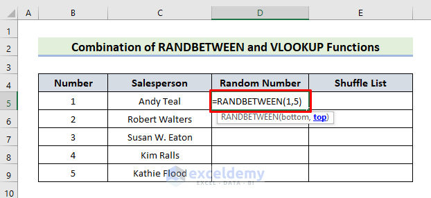
Enter the following RANDBETWEEN formula in cell D5:

=RANDBETWEEN(1,5)

These arguments can be integers or fractions but they always return an integer as output. The bottom represents the lowest number whereas the top function indicates the highest number between the given 2 numbers.
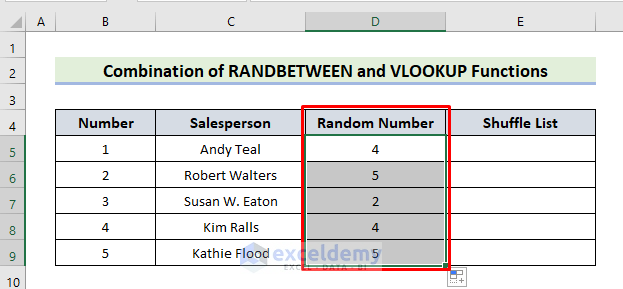
Press Enter to execute the formula.

A random number between 1 to 5 will be displayed in cell D5.
Drag the cell down to autofill the whole column with random numbers.

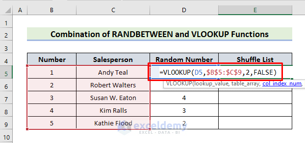
In the cell E5, enter the following VLOOKUP formula:

=VLOOKUP(D5,$B$5:$C$9,2, FALSE)

D5 is under the lookup argument that we will look for in column C. The argument $B$5:$C$9 is the array from where we will extract the value. The FALSE argument is under Range_lookup syntax that represents an exact match.
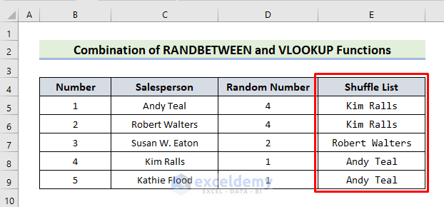
Press Enter.

Use the Autofill Handle for the remaining cells.

Method 2 – Combining RAND Function and Sort Feature to Shuffle Data

The RAND function returns evenly distributed random values from 0 to 1. The Sort feature sorts a range of cells in ascending or descending order according to a specific column. We will combine these 2 functions to shuffle the data.

Steps:

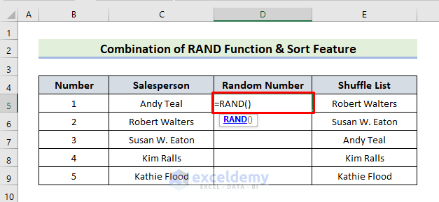
Enter the following code in D5:

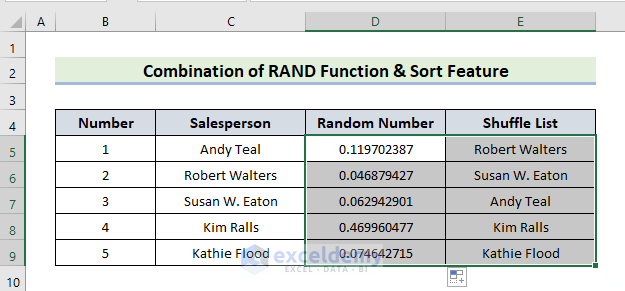
=RAND()

The RAND function will return a number from 0 to 1.
Use the Autofill Handle tool for the remaining cells.

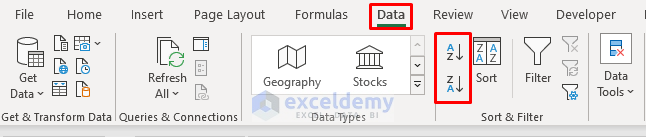
Select range D5:E9 to sort.

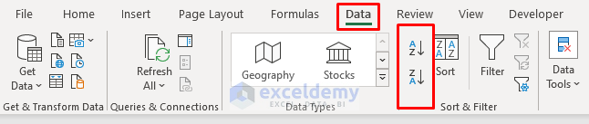
Go to the Data tab and locate Sort & Filter group.
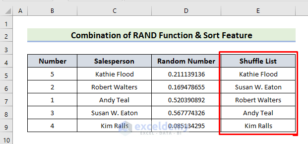
Click A-Z or Z-A to sort the data in ascending or descending order respectively.

The data will be sorted.

Method 3 – Mixing Data with Excel SORTBY Function

Steps:

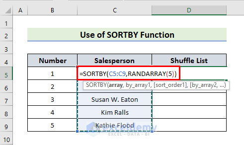
Enter the following formula in cell D5:

=SORTBY(C5:C9,RANDARRAY(5))

SORTBY sorts the array returned by the RANDARRAY and RANDARRAY(5) indicates the total number of data in the dataset.
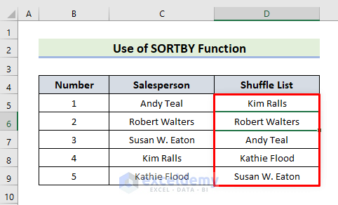
Press Enter to see the result.

Autofill the column by dragging the formula cell down.
You will get the desired result.

Method 4 – Inserting RANDBETWEEN Function for Shuffling Data

Steps:

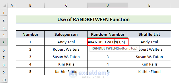
In cell D5, enter the following formula:

=RANDBETWEEN(1,5)

1 and 5 fall under the bottom and top arguments.
Press Enter to obtain random numbers from 1 to 5.

We will implement the Sort feature to mix up the data.
Go to the Data tab and select either A-Z or Z-A in the Sort group.

The result will be displayed in column E.

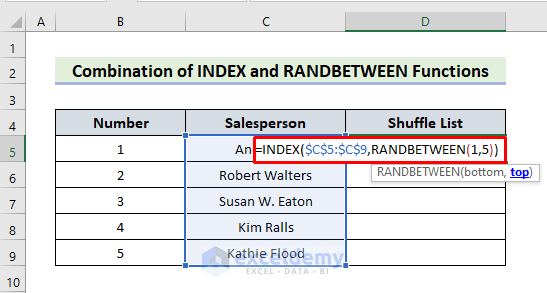
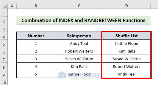
Method 5 – Randomizing Data with INDEX and RANDBETWEEN in Excel

We will combine the INDEX function and RANDBETWEEN function. The INDEX function returns a reference from a particular row or column.

Steps:

Enter the following formula in cell C5:

=INDEX($C$5:$C$9,RANDBETWEEN(1,5))

The RANDARRAY(1,5) will provide integer values randomly from 1 to 5.
The INDEX function will return the cell references of the random numbers.

Press Enter to get the result.

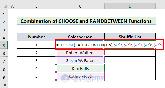
Method 6 – Joining CHOOSE & RANDBETWEEN Functions

The CHOOSE function returns a value using an index from a specific list.

Steps:

Enter the formula in cell D5:

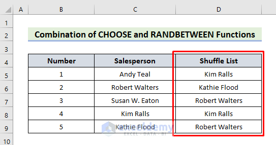
=CHOOSE(RANDBETWEEN(1,5),$C$5,$C$6,$C$7,$C$8,$C$9)

Press Enter.

The shuffled data will be shown in the dataset.

How Does the Formula Work?

RANDBETWEEN(1,5)

This part returns random numbers between two arrays called bottom and top. 1 and 5 indicate the bottom and top arrays that we want to calculate and later return 5 values. These values can be number or cell references.

CHOOSE(RANDBETWEEN(1,5),$C$5,$C$6,$C$7,$C$8,$C$9)

$C$5 returns as Value1, $C$6 returns as Value2 and so on. They return the cell references from where the CHOOSE function will specify the range. The CHOOSE function specifies the range using the cell references and returns values using the index.

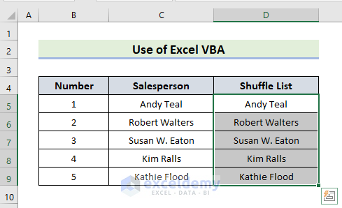
Method 7 – Shuffling Data Through Excel VBA

We will use the Excel VBA to randomize data. We will use a simple VBA code that receives the currently selected cell information, for instance, font color, background color, etc. Later, it will shuffle them into the dataset.

Steps:

Select the range D5:D9.
Go to Developer > Visual Basic > Insert > Module.
A module box will pop up.

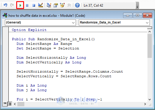
In the module box, enter the following VBA code.

Option Explicit
Public Sub Randomize_Data_in_Excel()
  Dim SelectRange As Range
  Set SelectRange = Selection
  Dim SelectHorizontally As Long
  Dim SelectVertically As Long
  SelectHorizontally = SelectRange.Columns.Count
  SelectVertically = SelectRange.Rows.Count
  Dim i As Long
  Dim j As Long
  For i = SelectVertically To 1 Step -1
    For j = SelectHorizontally To 1 Step -1
      Dim RandomRow As Long
      Dim RandomColumn As Long
      RandomRow = Application.WorksheetFunction.RoundDown(SelectVertically * Rnd + 1, 0)
      RandomColumn = Application.WorksheetFunction.RoundDown(SelectHorizontally * Rnd + 1, 0)
      Dim temp As String
      Dim tempColor As Long
      Dim tempFontColor As Long
      temp = SelectRange.Cells(i, j).Formula
      tempColor = SelectRange.Cells(i, j).Interior.Color
      tempFontColor = SelectRange.Cells(i, j).Font.Color
      SelectRange.Cells(i, j).Formula = SelectRange.Cells(RandomRow, RandomColumn).Formula
      SelectRange.Cells(i, j).Interior.Color = SelectRange.Cells(RandomRow, RandomColumn).Interior.Color
      SelectRange.Cells(i, j).Font.Color = SelectRange.Cells(RandomRow, RandomColumn).Font.Color
      SelectRange.Cells(RandomRow, RandomColumn).Formula = temp
      SelectRange.Cells(RandomRow, RandomColumn).Interior.Color = tempColor
      SelectRange.Cells(RandomRow, RandomColumn).Font.Color = tempFontColor
    Next j
  Next i
End Sub