Method 1 – Utilizing Sort Feature
Steps:
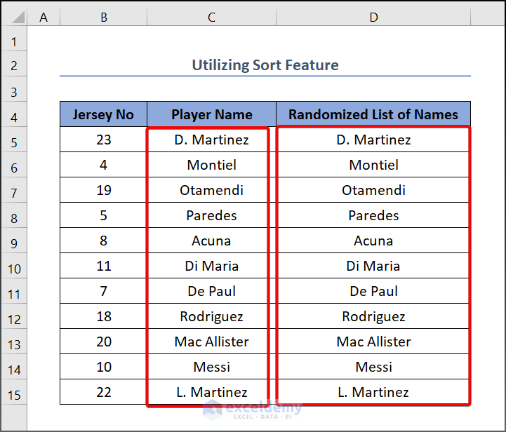
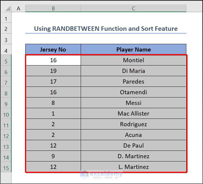
- Select the entire dataset for which you want to do your task.
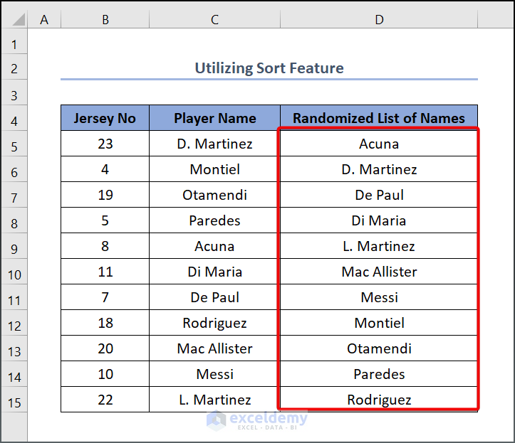
- We copied C5:C15 data in D5:D15. Randomize the copied data in the same D5:D15 cell.
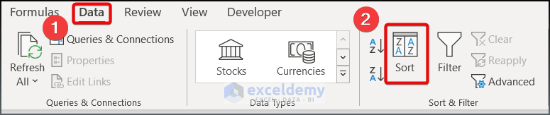
- Click the Data tab.
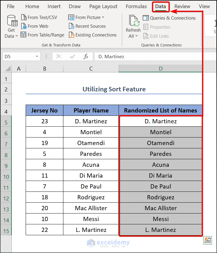
- Proceed to the Sort command.
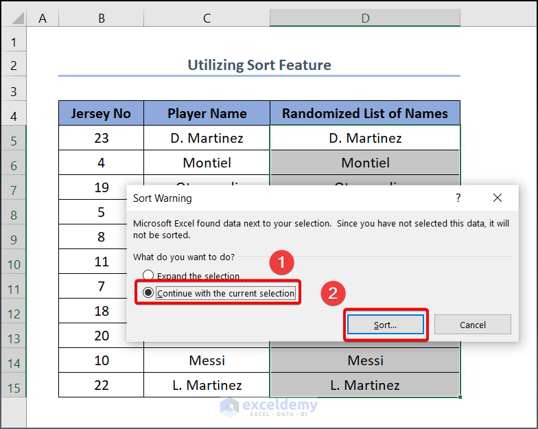
- A prompt will pop up where we select Continue with the current selection.
- Click the Sort button.
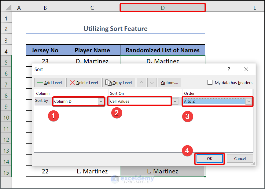
- In the Sort by option, select the name of the column if it does not appear automatically. In our case, our intended data was in Column D.
- Select Cell Values and A to Z as described below.
- Press OK.
- Our output will look like the one given below.
Method 2 – Using RANDBETWEEN Function and Sort Feature
Steps:
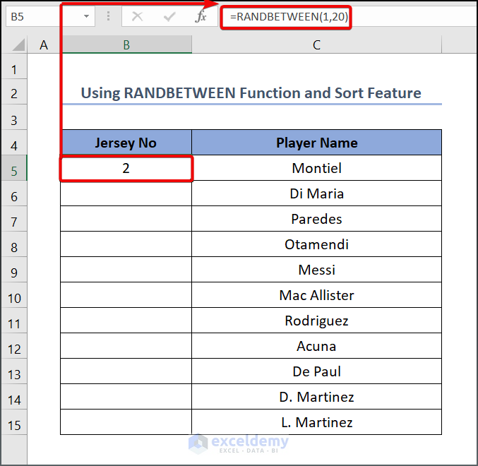
- Enter the following formula in cell B5.
=RANDBETWEEN(1,20)- The function will generate some random number between 1 to 20.
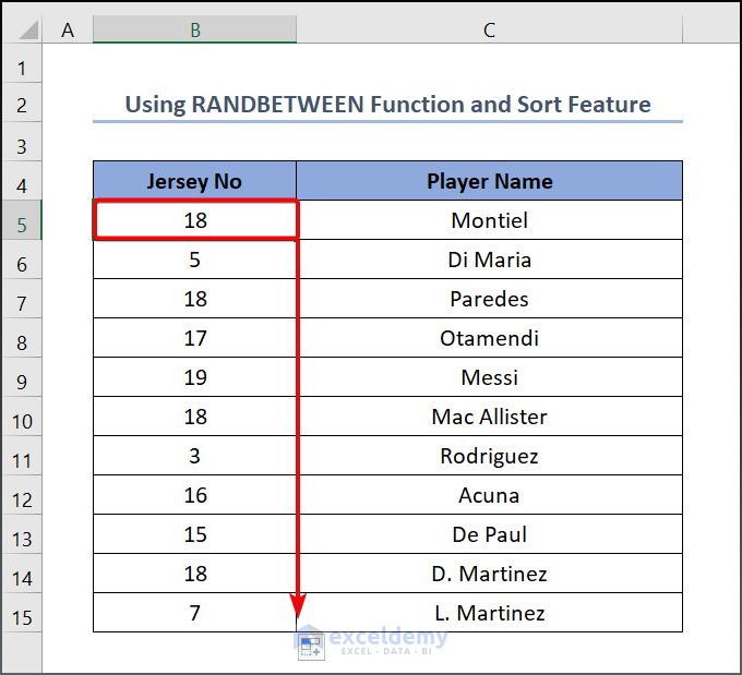
- Drag the Fill Handle tool from B5 to B15 to get the rest of the value.
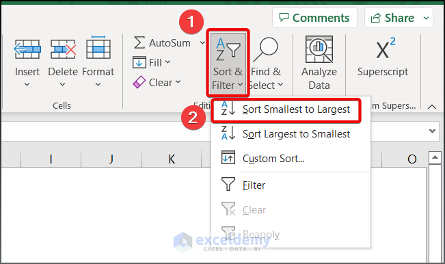
- Select the range of your data (B5:C15 in our case)
- Click the Home tab > Editing group > Sort & Filter button > Sort Smallest to Largest (any of the two options will work).
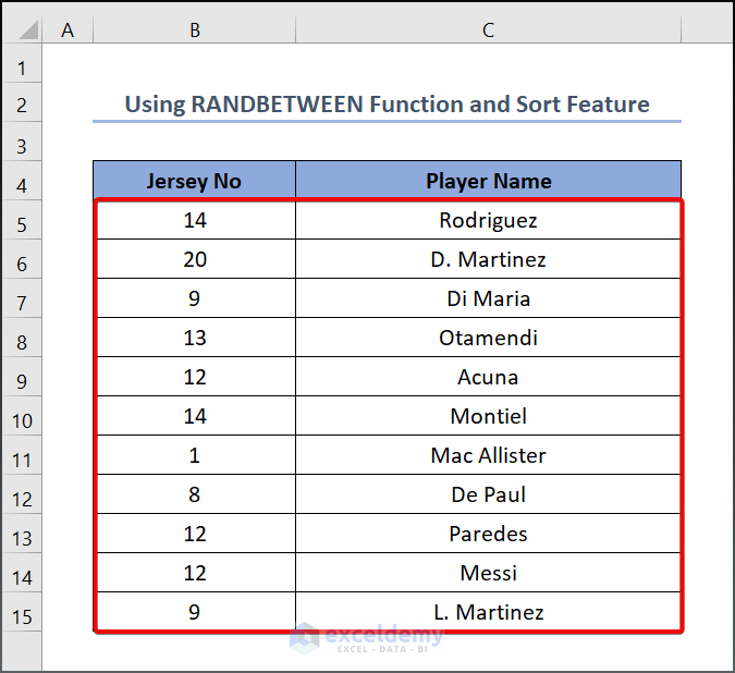
- See the output given below.
Method 3 – Using SORTBY Function
Steps:
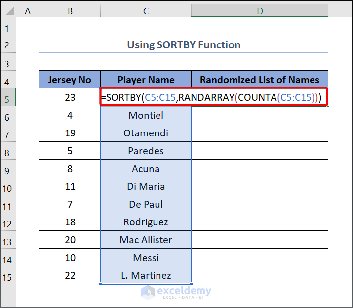
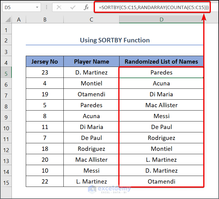
- Write the following formula in cell D5.
=SORTBY(C5:C15,RANDARRAY(COUNTA(C5:C15)))Formula Explanation:
The COUNTA function returns the number of cells from the C5:C15 cell range containing any text values. The RANARRAY function generates an array of random numbers, with the row numbers determined by the output of COUNTA(C5:C15). The SORTBY function performs sorting based on the output of the RANDARRAY function.
- Press Enter.
- See the output below.
Method 4 – Applying the Combination of SORTBY and RANDARRAY Functions
Steps:
- Write the following formula in cell D5.
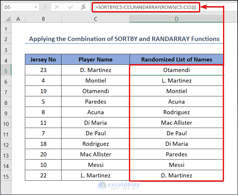
=SORTBY(C5:C15,RANDARRAY(ROWS(C5:C15)))The ROWS(C5:C15) syntax returns the number of rows.
- Press Enter.
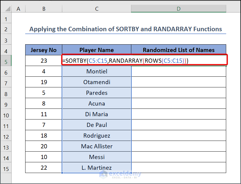
- See the output below.
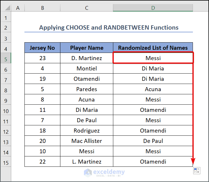
Method 5 – Applying CHOOSE and RANDBETWEEN Functions
Steps:
- Write the following formula in cell D5.
=CHOOSE(RANDBETWEEN(5,12),$C$3,$C$4,$C$5,$C$6,$C$8,$C$7,$C$9,$C$10,$C$11,$C$12,$C$13,$C$14)Formula Explanation:
- RANDBETWEEN(5,12) returns a random value starting from 5 to 12.
- The values followed by RANDBETWEEN assign the number to the individual Player Name using absolute cell reference.
- The CHOOSE function returns the value from the input data to the created number.
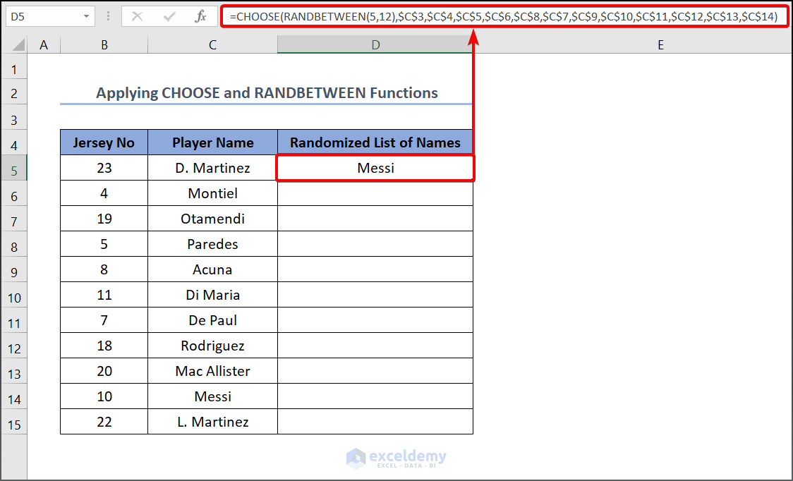
- Drag the Fill Handle tool from D5 to D15.
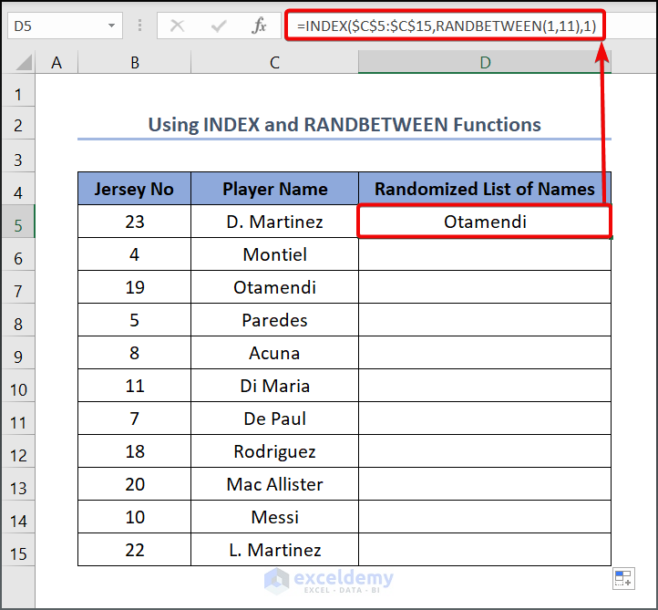
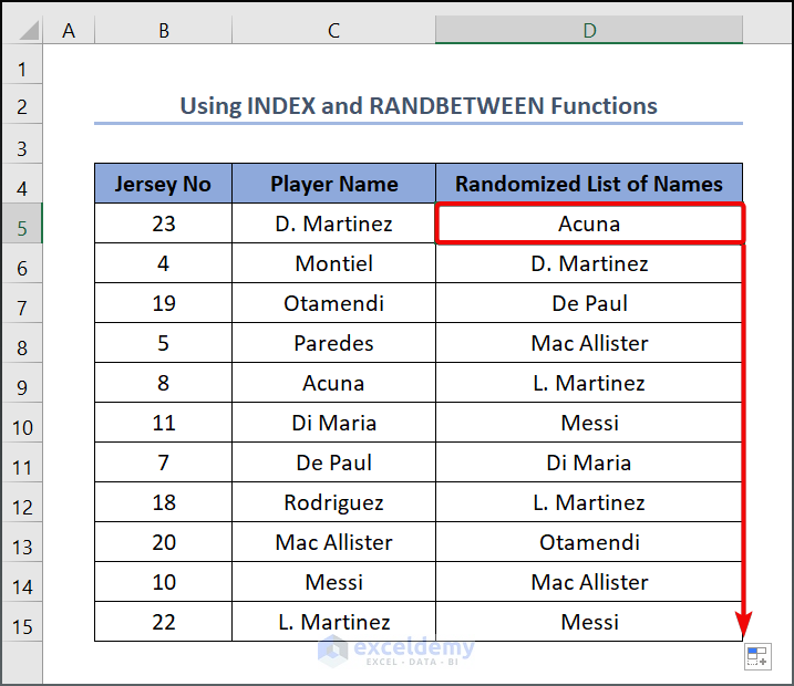
Method 6 – Using INDEX and RANDBETWEEN Functions
Steps:
- Enter the following formula in cell D5.
=INDEX($C$5:$C$15,RANDBETWEEN(1,11),1)The RANDBETWEEN function randomly returns a number from 1 to 11. In our first case, 1 is the initial number. This unique value will be used as an index number and referred to as the corresponding cell value in the respective cell.
- Drag the Fill Handle tool from D5 to D15. So here is our output given below.
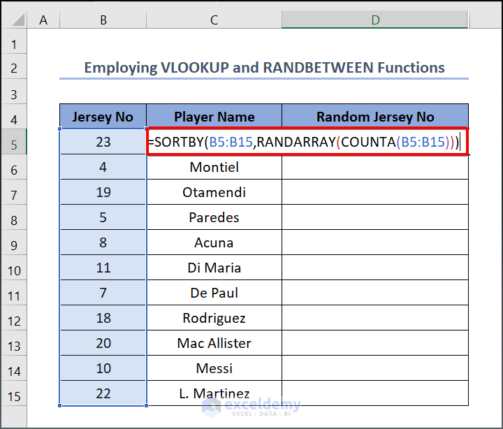
Method 7 – Employing VLOOKUP and RANDBETWEEN Functions
Steps:
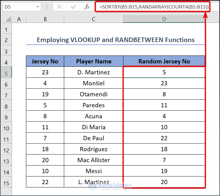
- Generate a number to attribute our “Player Name”, type the following formula in cell D5.
=SORTBY(B5:B15,RANDARRAY(COUNTA(B5:B15)))- Press Enter.
- The output is below.
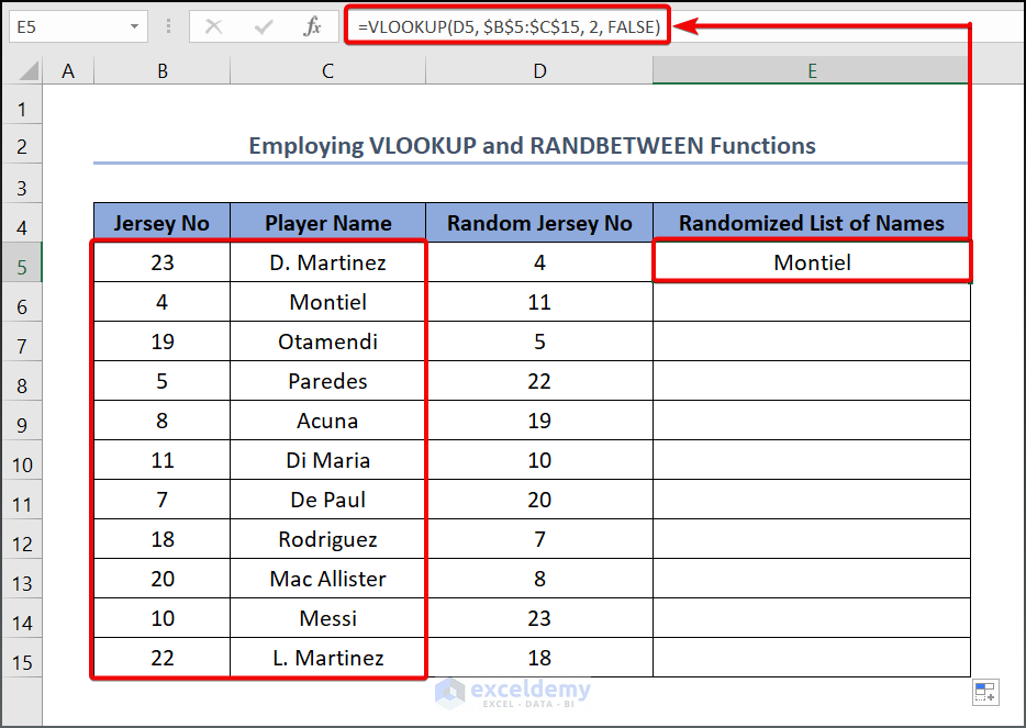
- Enter the following formula in cell E5.
=VLOOKUP(D5, $B$5:$C$15, 2, FALSE)D5 is the lookup value, B5:C15 is the table array, 2 is the column index number as the lookup value is in the 2nd column from Column B, and FALSE is for exact matching.
Note: We used the dollar sign ($) to fix the cell range while using the Fill Handle tool for copying the formula to the rest cells.
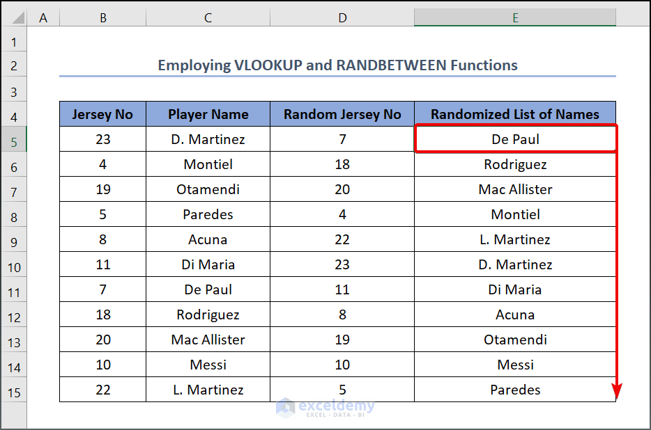
- Drag the Fill Handle tool to get the other value.
Method 8 – Incorporating the Power Query Feature
Steps:
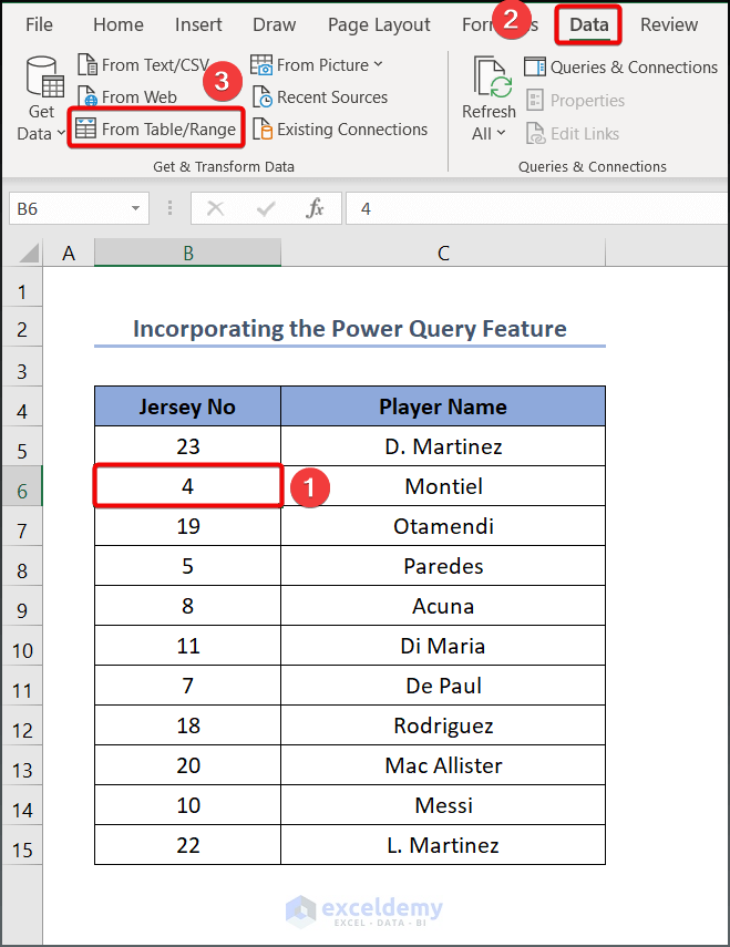
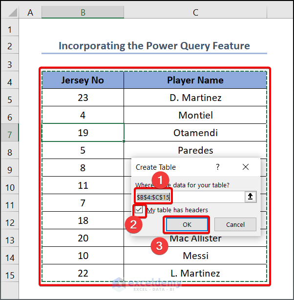
- Select any cell inside your data.
- Go to the Data tab > From Table/Range command.
- A prompt will appear and ask you to create a table. Select your data area, $B$4:$C15$ for instance.
- Press OK.
- Double-click on the region denoted by 1 and name the sheet where you want your output to appear.
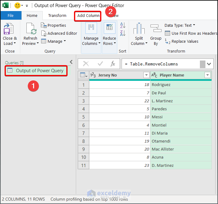
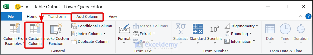
- Click Add Column > Custom Column command.
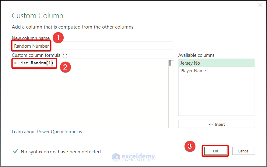
- Add a name such as Random Number in the New column name box.
- Type the following formula into the Custom Column Formula editor.
= List.Random(1)Each row gets a list as a result. You must extract the values from each list’s single random number, which ranges from 0 to 1, to utilize them to sort the data.
- Click OK.
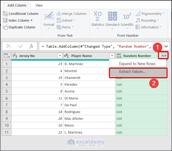
- Click the Filter toggle in the Random Number column, which contains all the List items.
- Select the Extract values option.
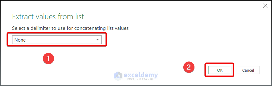
- Select None > OK button.
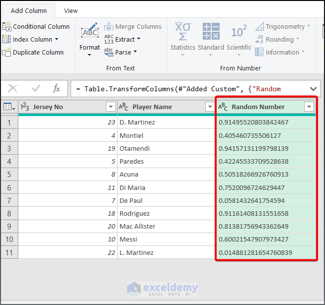
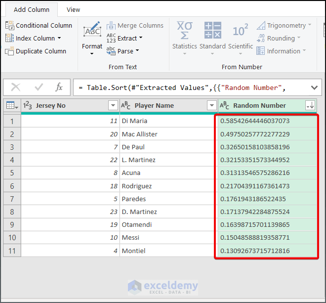
- A random number will be generated as below.
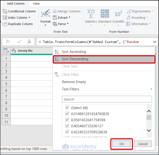
- Click on the Filter toggle in the Random Number
- Choose either the Sort Ascending or Sort Descending, we choose Sort Descending option.
- Press OK.
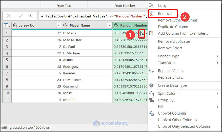
- The Random Number column is no longer required because the data has already been sorted based on it, so you can delete it.
- To delete those numbers, right-click on the Random Number column heading containing the random numbers.
- Select the Remove option from the menu.
- Go to the Home tab and select the Close & Load option.

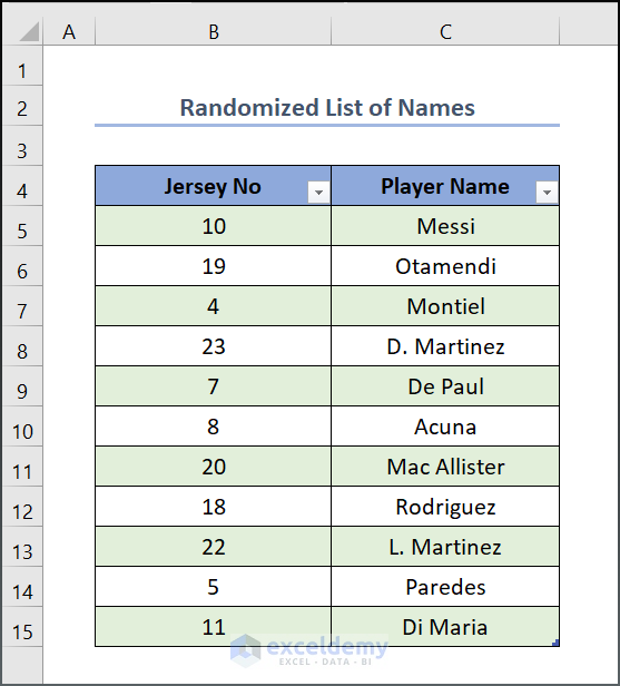
- See the output given below now.
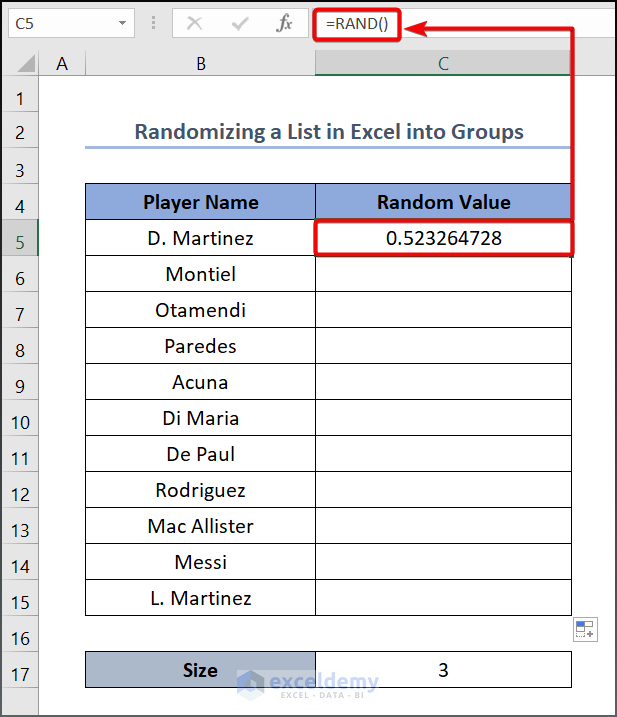
How to Randomize a List into Groups in Excel
Steps:
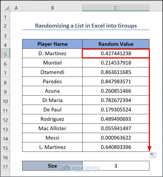
- Assign some random values in column C by using the RAND function.
- Drag the Fill Handle tool.
- Type the following formula in cell D5.
=ROUNDUP(RANK(C5, C5:C15)/$C$17,0)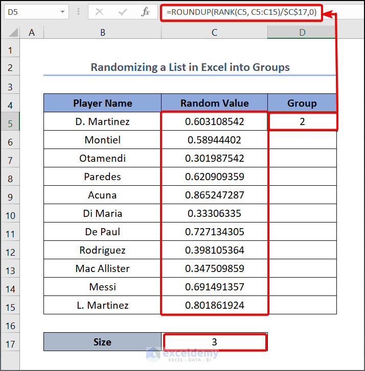
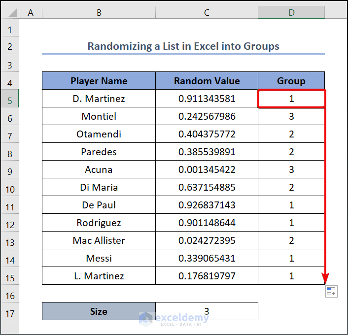
- Drag the Fill Handle tool to get the other value.
Download Practice Workbook
<< Go Back to Randomize in Excel | Learn Excel
Get FREE Advanced Excel Exercises with Solutions!

