Method 1 – Randomize a List in Excel Into Groups Using RAND Function
Steps:
- Select the C5 cell and copy the following formula into it.
=RAND()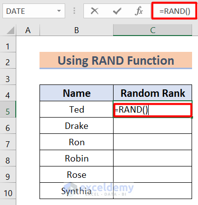
- Enter, you will find the following number.
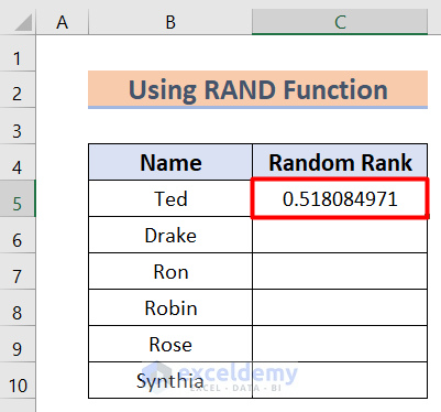
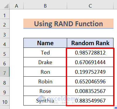
- Fill Handle the formula to copy down from C5 to C10.
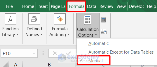
- Go to the Formula tab in your toolbar.
- Select the Calculation option.
- Select the manual option.
- Select the Home tab and go to the Editing option.
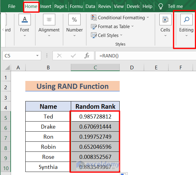
- Select the Sort and Filter option.
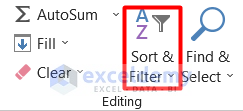
- A pop-up window will appear. Select the Sort Largest to Smallest option.
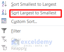
- Select the Expand the Selection option and select the Sort button.

- Excel will sort the Names like the following picture.
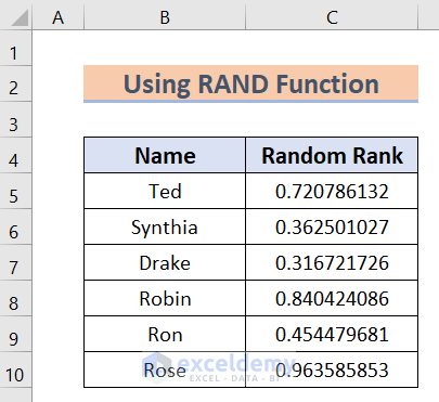
This is how the randomization of a list can happen.
Method 2 – Implementing Excel RANDBETWEEN Function to Randomize a List
Steps:
- Select the C5 cell.
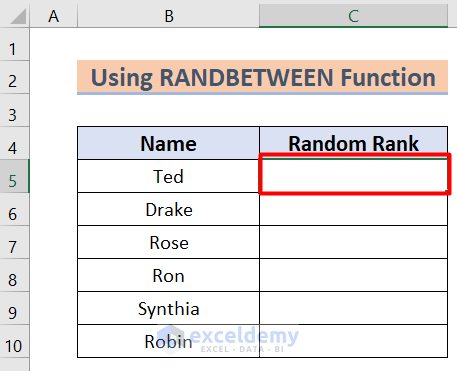
- Copy down the following formula in the selected cell.
=RANDBETWEEN(1,6)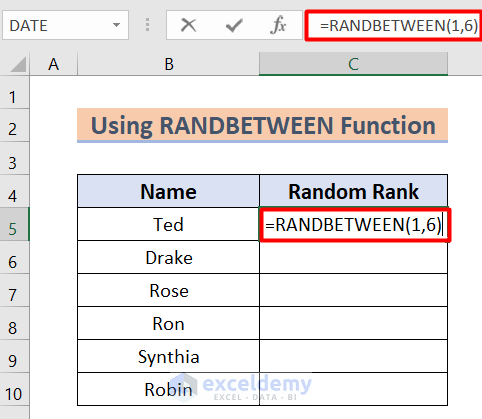
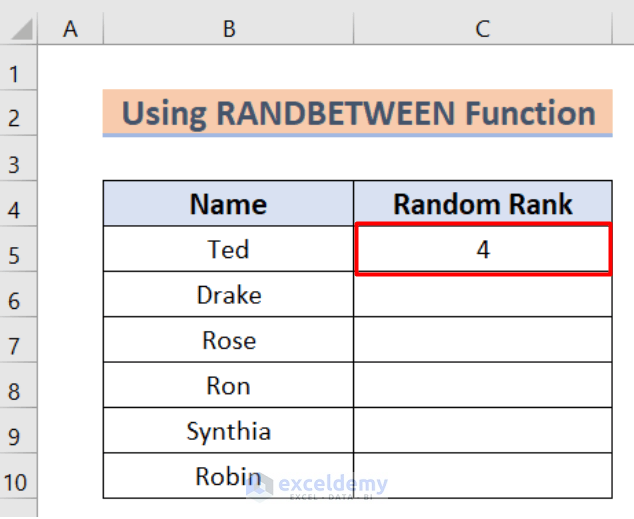
- After pressing Enter, Excel will show the following result.
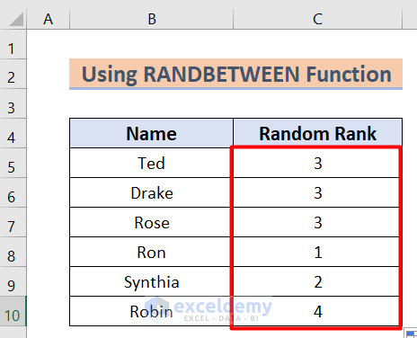
- Copy down the formula to the C10 cell.
- You will get random numbers like the picture given below.
- To stop the automatic changing of the numbers, go to the Formulas tab and select the Calculation Options.
- Select the Manual option.

- Go to the Home tab and select the Editing option.
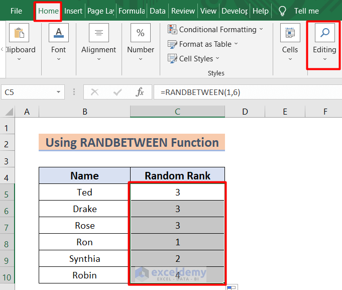
- Select the Sort & Filter option.

- Select the Sort Largest to Smallest option.

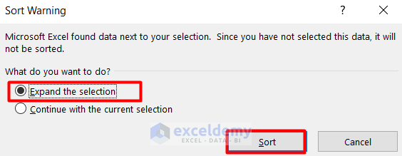
- Meanwhile, the following window will appear. Select the Expand the selection option and then press the Sort button.
- As a result, Excel will show the following sorted result.
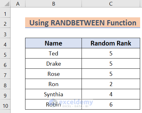
This is how you can use the RANDBETWEEN function to randomize Excel lists.
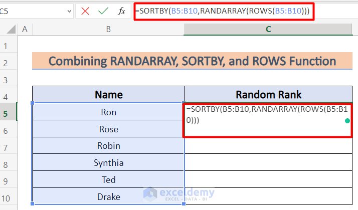
Method 3 – Combine RANDARRAY, SORTBY, and ROWS Functions
Steps:
- Select the C5 cell.
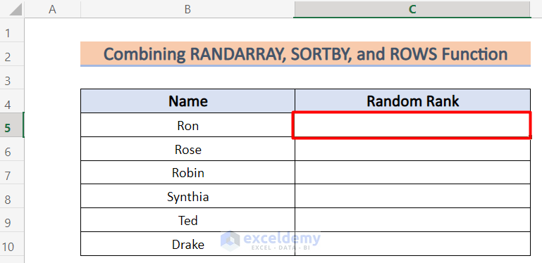
- Copy the following formula in the selected cell.
=SORTBY(B5:B10,RANDARRAY(ROWS(B5:B10)))- ROWS(B5:B10): Returns the row numbers of the array.
- RANDARRAY(ROWS(B5:B10): Returns an Array according to the ROWS
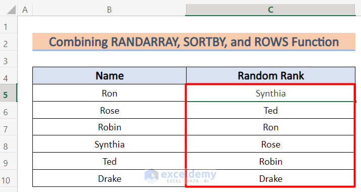
- SORTBY(B5:B10, RANDARRAY(ROWS(B5:B10))): Returns the newly sorted names and spills the names throughout the whole column.
- Pressing Enter, Excel will show the following result.
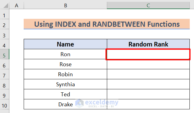
Method 4 – Using INDEX and RANDBETWEEN Functions
Steps:
- Select the C5 cell first.
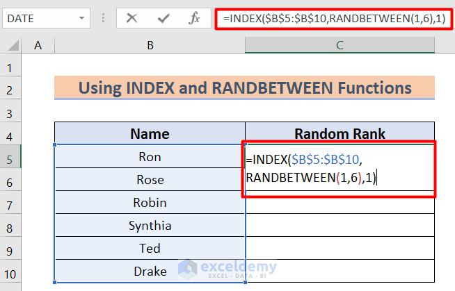
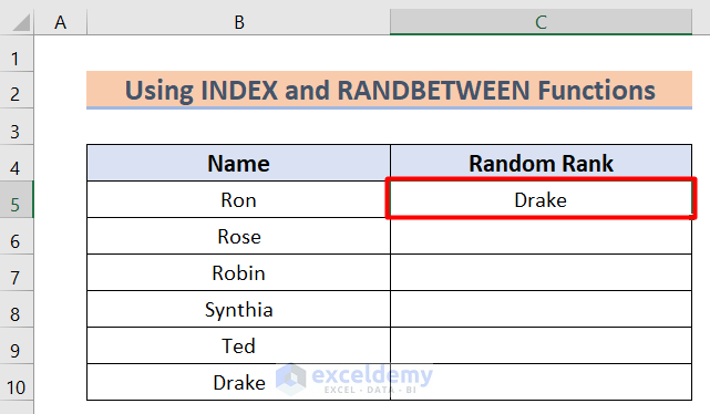
- Write down the following formula in the selected cell.
=INDEX($B$5:$B$10,RANDBETWEEN(1,6),1)- RANDBETWEEN(1,6): Returns a random number in a cell between 1 to 6.
- INDEX($B$5:$B$10, RANDBETWEEN(1,6),1): Returns randomly sorted names in a certain cell.
- The following result will be shown.
- Excel will show the following result.
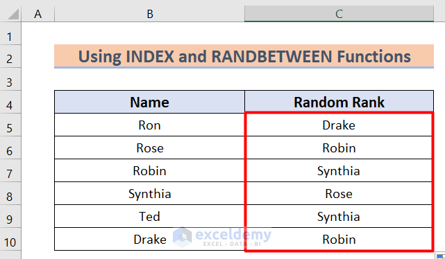
We can randomize a list in Excel using the INDEX and RANDBETWEEN Functions.
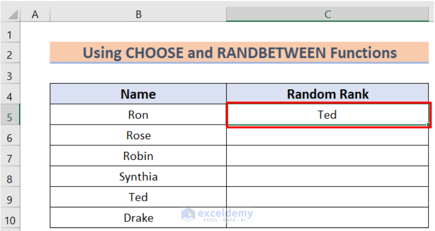
Method 5 – Applying CHOOSE and RANDBETWEEN Functions
Steps:
- Select the C5 cell first.
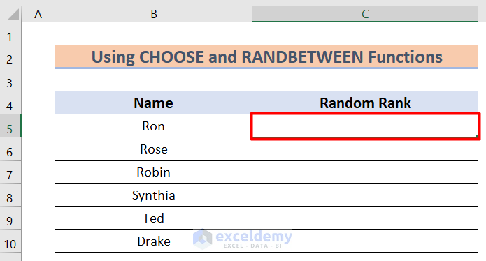
- Write down the following formula in the selected cell.
=CHOOSE(RANDBETWEEN(1,6),$B$5,$B$6,$B$7,$B$8,$B$9,$B$10)- CHOOSE(RANDBETWEEN(1,6),$B$5,$B$6,$B$7,$B$8,$B$9,$B$10): Returns the shuffled names in the C column.
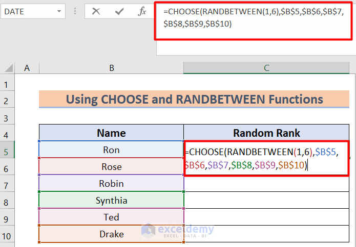
- After pressing Enter, the following result will be shown.
- Copy down the formula from C5 to C10
- The following result will be found.
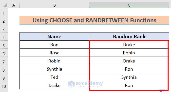
This is the procedure how to randomize a list in Excel into groups.
Things to Remember
- You should bear in mind that the SORTBY function can only be found in Excel 365.
Download Practice Workbook
<< Go Back to Randomize in Excel | Learn Excel
Get FREE Advanced Excel Exercises with Solutions!
