Method 1 – Randomizing Rows in Excel with Multiple Columns
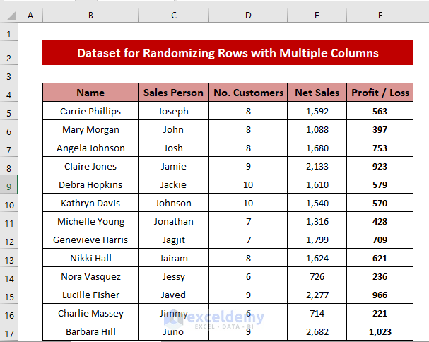
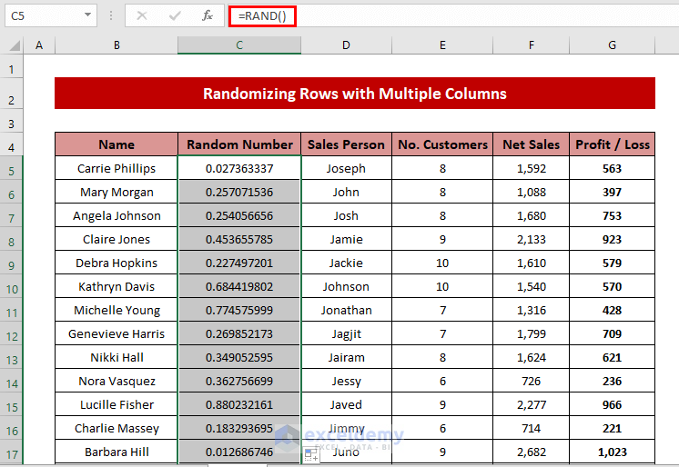
We have a dataset of some sales representatives of an organization, their net sales, profits, and the number of customers they had over a certain period of time.
Steps:
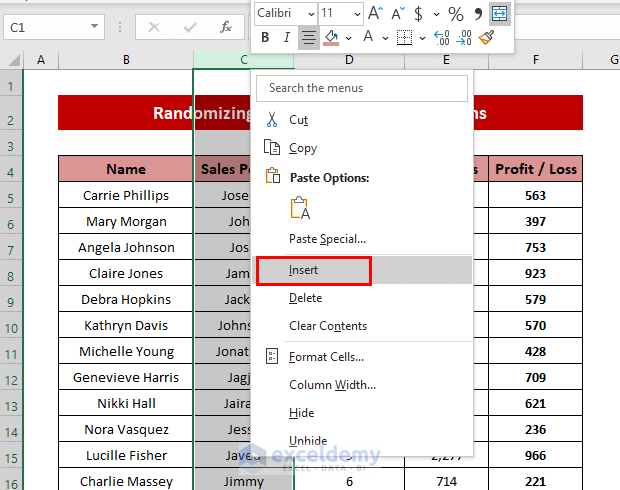
- Click the header letter of column B, and the whole B column will be selected.
- Right-click and choose the Insert command, and a new column will be created.
- Select the first cell (i.e. C5) in the column and use the following formula into the cell.
=RAND()The RAND function returns a random number between 0 and 1, not including 1.
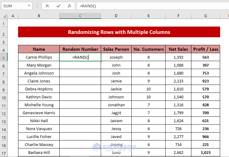
- Press Enter.
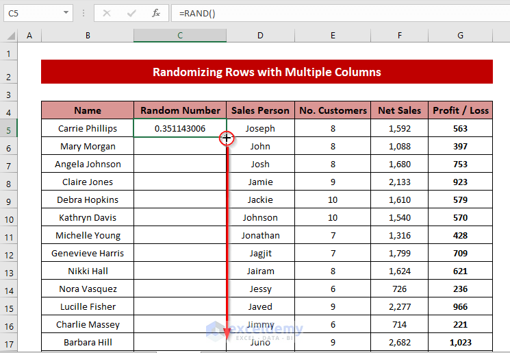
- Select the cell C5 again and you will see the Fill Handle tool on the bottom-right corner.
- Click on the Fill Handle and drag the tool down the next cells to Autofill the formula until you have reached the last cell of the column.
- Alternatively, while clicking cell C5, press Shift and use the Navigation Down Arrow (⇓) to reach the last cell, then press Ctrl + D to Autofill.
- Every time you make any change to the worksheet, the random numbers will change their value.
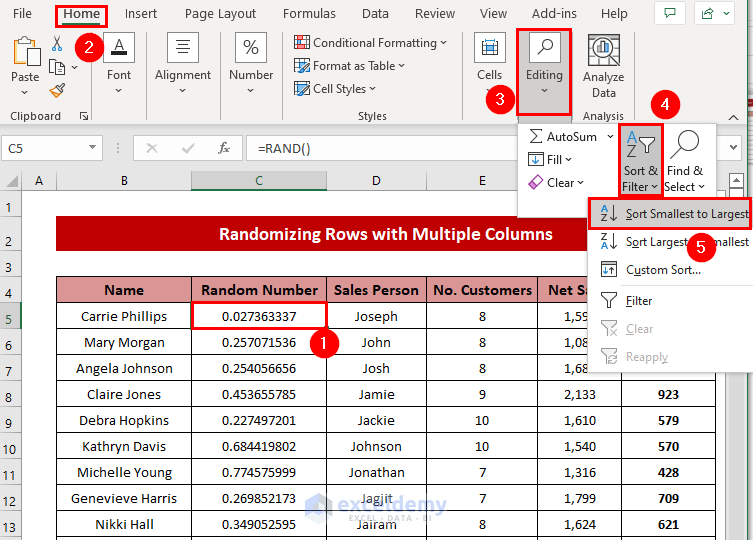
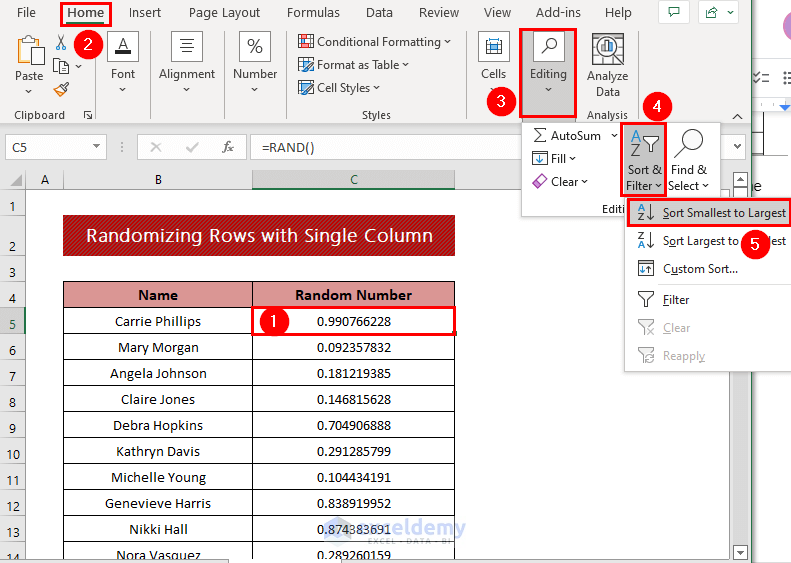
- Select cell C5 again.
- Go to the Home tab, click on Sort & Filter in the Editing group, and select Sort Smallest to Largest.
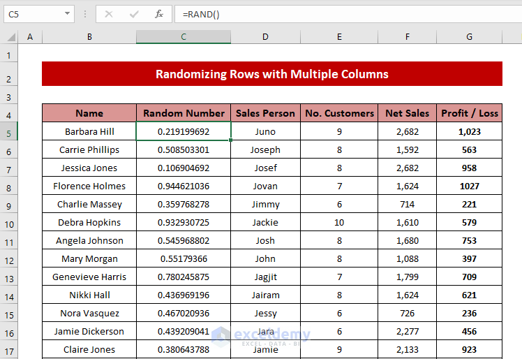
- Your rows will randomize themselves. All the columns have also been randomly changed alongside the rows.
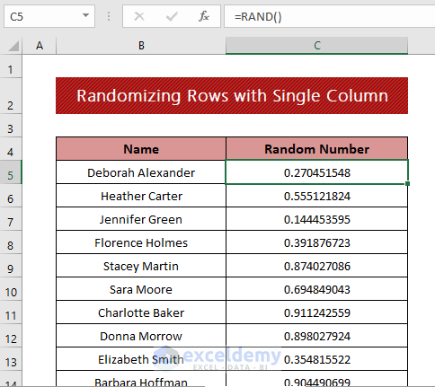
Method 2 – Randomizing Rows with a Single Column in Excel
Steps:
- Enter the RAND function in cell C5 just like Method 1.
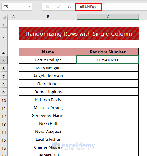
- Drag and Autofill the formula.
- Go to the Home, click Sort & Filter, and select Sort Smallest to Largest.
- The order of names will be randomized.
How to Shuffle Rows in Excel
Steps:
- Create a new column and use the following formula to the first cell of the column.
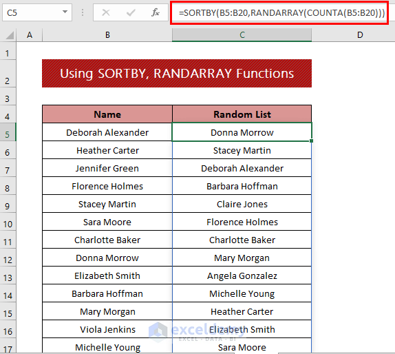
=SORTBY(B5:B20,RANDARRAY(COUNTA(B5:B20)))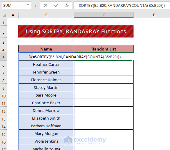
💡 Formula Breakdown
COUNTA(B5:B20) returns the number of cells in the lookup array (B5:B20)
Output=> 16.
RANDARRAY(16) gives 16 random numbers for the 16 cells.
Finally, SORTBY(B5:B20,RANDARRAY(16))) will shuffle the cells along the rows with the random values.
- Press Enter, and the values get shuffled.
Download the Practice Workbook
<< Go Back to Randomize in Excel | Learn Excel
Get FREE Advanced Excel Exercises with Solutions!
