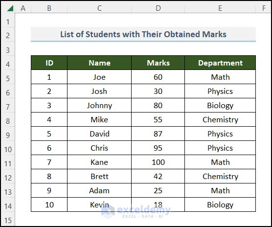
Let’s use a List of Students with Their Obtained Marks. This dataset contains the ID, Name, and their corresponding Marks and Departments in columns B, C, D, and E, respectively.
Method 1 – Implementing Array Formula to Extract Data Based on Range Criteria from Excel
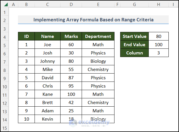
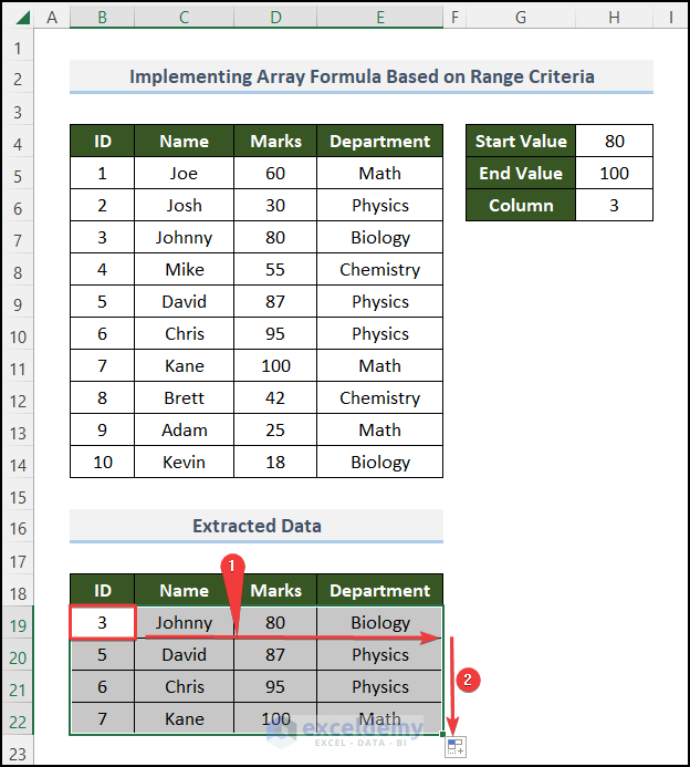
Let’s retrieve the student details for students who got Marks from 80 to 100.
Steps:
- Store the condition in other cells to work with those later. We stored 80 as the Start Value and 100 as the End Value in cells H4 and H5 respectively. Since the Marks column which is the 3rd column in our dataset, we stored 3 as the Column value in cell H6.
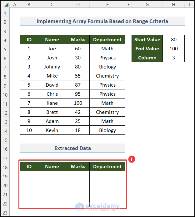
- Make an output range in cells in the B18:E22 range.
- In the first cell where you want the result (we wanted our result in cell B19), write the following formula:
=INDEX($B$5:$E$14,SMALL(IF((INDEX($B$5:$E$14,,$H$6)<=$H$5)*(INDEX($B$5:$E$14,,$H$6)>=$H$4),MATCH(ROW($B$5:$E$14),ROW($B$5:$E$14)),""),ROWS(B19:$B$19)),COLUMNS($A$1:A1))Formula Breakdown
- INDEX($B$5:$E$14,,$H$6)
- Output: {60;30;80;55;87;95;100;42;25;18}
- Explanation: The INDEX Function usually returns a single value or an entire column or row from a given cell range. 3 is stored in the Cell $H$6, so it returns the entire column no 3 (Marks column) from the whole range of the dataset ($B$5:$E$14) as output.
- INDEX($B$5:$E$14,,$H$6)<=$H$5 -> becomes,
- {60;30;80;55;87;95;100;42;25;18}<=100
- Output: {TRUE;TRUE;TRUE;TRUE;TRUE;TRUE;TRUE;TRUE;TRUE;TRUE}
- Explanation: We stored 100 in the Cell $H$5. As all of the values are less than 100 ($H$5), so it returns a column full of TRUE.
Similarly,
- INDEX($B$5:$E$14,,$H$6)>=$H$4 -> becomes,
- {60;30;80;55;87;95;100;42;25;18}>=80
- Output: {FALSE;FALSE;TRUE;FALSE;TRUE;TRUE;TRUE;FALSE;FALSE;FALSE}
- Explanation: We stored 80 in the Cell $H$4. So it returns TRUE when the value from the column is equal or greater than 80; otherwise, it returns FALSE.
- (INDEX($B$5:$E$14,,$H$6)<=$H$5)*(INDEX($B$5:$E$14,,$H$6)>=$H$4) -> becomes,
- {TRUE;TRUE;TRUE;TRUE;TRUE;TRUE;TRUE;TRUE;TRUE;TRUE}*{FALSE;FALSE;TRUE;FALSE;TRUE;TRUE;TRUE;FALSE;FALSE;FALSE}
- Output: {0;0;1;0;1;1;1;0;0;0}
- Explanation: Boolean values have numerical equivalents, TRUE = 1 and FALSE = 0 (zero). They are converted when performing an arithmetic operation in a formula.
- ROW($B$5:$E$14)
- Output: {5;6;7;8;9;10;11;12;13;14}
- Explanation: The ROW function calculates the row number of a cell reference.
- MATCH(ROW($B$5:$E$14),ROW($B$5:$E$14)) -> becomes,
- MATCH({5;6;7;8;9;10;11;12;13;14},{5;6;7;8;9;10;11;12;13;14})
- Output: {1; 2; 3; 4; 5; 6; 7; 8; 9; 10}
- Explanation: The MATCH function returns the relative position of an item in an array or cell reference that matches a specified value in a specific order.
- IF((INDEX($B$5:$E$14,,$H$6)<=$H$5)*(INDEX($B$5:$E$14,,$H$6)>=$H$4),MATCH(ROW($B$5:$E$14),ROW($B$5:$E$14)),””) -> becomes,
- IF({0;0;1;0;1;1;1;0;0;0}),{1; 2; 3; 4; 5; 6; 7; 8; 9; 10},””)
- Output: {“”; “”; 3; “”; 5; 6; 7; “”; “”; “”}
- Explanation: The IF function returns one value if the logical test is TRUE and another value if the logical test is FALSE.
- SMALL(IF((INDEX($B$5:$E$14,,$H$6)<=$H$5)*(INDEX($B$5:$E$14,,$H$6)>=$H$4),MATCH(ROW($B$5:$E$14),ROW($B$5:$E$14)),””),) -> becomes,
- SMALL({“”; “”; 3; “”; 5; 6; 7; “”; “”; “”},ROWS(B19:$B$19)) -> becomes,
- SMALL({“”; “”; 3; “”; 5; 6; 7; “”; “”; “”},1)
- Output: 3
- Explanation: The SMALL function returns the k-th smallest value from a group of numbers. 3 is the smallest in this group.
- INDEX($B$5:$E$14,SMALL(IF((INDEX($B$5:$E$14,,$H$6)<=$H$5)*(INDEX($B$5:$E$14,,$H$6)>=$H$4),MATCH(ROW($B$5:$E$14),ROW($B$5:$E$14)),””),ROWS(B19:$B$19)),COLUMNS($A$1:A1)) -> becomes,
- INDEX($B$5:$E$14,3,,1)
- Output: {3; “Johnny”, 80, “Biology”}
- Explanation: The INDEX function returns a value from a cell range($B$5:$E$14), specified by the value based on a row and column number.
- Press Enter on your keyboard.
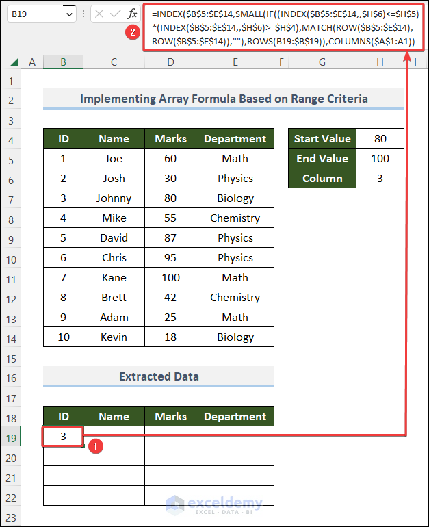
Then, you will get the first extracted data that matches your condition in the result cell. E.g. Johnny whose ID is 3 got 80 marks in Biology and his record is stored in the dataset first, so we got Johnny’s ID 3 in the first result cell (cell B19).
- Drag around the columns and rows via the Fill Handle to cover the rest of the range.
Read More: How to Extract Data from Cell in Excel
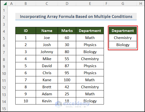
Method 2 – Incorporating Array Formula to Extract Data from Excel Based on Multiple Conditions
Look at the same dataset as before but here instead of storing a range of values (marks 80 to 100) as a condition, we stored multiple conditions such as retrieving students’ details from both Chemistry and Biology departments.
Steps:
- Store the conditions in other cells to work with those later. Since we’re extracting students’ details from the Chemistry and Biology departments, we stored Chemistry and Biology in cells G5 and G6 respectively.
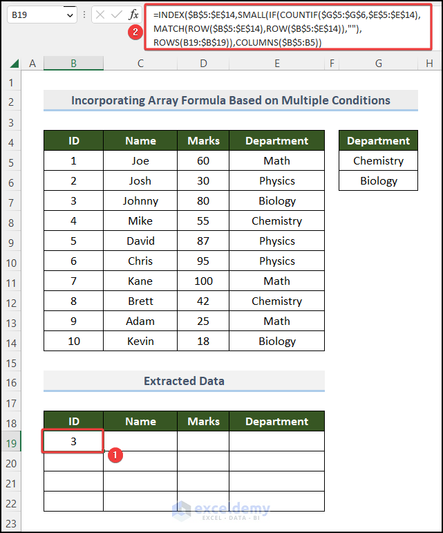
- In the first result cell (we wanted our result in cell B19), write the following formula:
=INDEX($B$5:$E$14,SMALL(IF(COUNTIF($G$5:$G$6,$E$5:$E$14),MATCH(ROW($B$5:$E$14),ROW($B$5:$E$14)),""),ROWS(B19:$B$19)),COLUMNS($B$5:B5))Formula Breakdown
- COUNTIF($G$5:$G$6,$E$5:$E$14) -> becomes,
- COUNTIF({“Chemistry”;“Biology”},{“Math”;“Physics”;“Biology”;“Chemistry”;“Physics”;“Physics”;“Math”;“Chemistry”;“Math”;“Biology”}
- Output: {0;0;1;1;0;0;0;1;0;1}
- Explanation: The COUNTIF function allows us to identify cells in the range $G$5:$G$6 that equals $E$5:$E$14.
- IF(COUNTIF($G$5:$G$6,$E$5:$E$14),MATCH(ROW($B$5:$E$14),ROW($B$5:$E$14)),””) -> becomes,
- IF({0;0;1;1;0;0;0;1;0;1},MATCH(ROW($B$5:$E$14),ROW($B$5:$E$14)),””) -> becomes,
- IF({0;0;1;1;0;0;0;1;0;1},{1; 2; 3; 4; 5; 6; 7; 8; 9; 10},””)
- Output: {“”; “”; 3; 4; “”; “”;“”; 8; “”;10}
- Explanation: The IF function has three arguments, the first one must be a logical expression. If the expression evaluates to TRUE then one thing happens (argument 2) and if FALSE another thing happens (argument 3). The logical expression was calculated in step 1, TRUE equals 1, and FALSE equals 0 (zero). Row no 3, 4, 8, and 10 evaluate TRUE (1).
- SMALL(IF(COUNTIF($G$5:$G$6,$E$5:$E$14),MATCH(ROW($B$5:$E$14),ROW($B$5:$E$14)),””),ROWS(B19:$B$19)) -> becomes,
- SMALL({“”; “”; 3; 4; “”; “”;“”; 8; “”;10},ROWS(B19:$B$19)) -> becomes,
- SMALL({“”; “”; 3; 4; “”; “”;“”; 8; “”;10},1)
- Output: 3
- Explanation: The SMALL function returns the k-th smallest value from a group of numbers. 3 is the smallest in this group.
- INDEX($B$5:$E$14, SMALL(IF(COUNTIF($G$5:$G$6,$E$5:$E$14),MATCH(ROW($B$5:$E$14),ROW($B$5:$E$14)),””),ROWS(B19:$B$19)),COLUMNS($B$5:B5)) -> becomes,
- INDEX($B$5:$E$14, 3, COLUMNS($B$5:B5)) -> becomes,
- INDEX($B$5:$E$14, 3, 1)
- Output: {3; “Johnny”, 80, “Biology”}
- Explanation: The INDEX function returns a value from a cell range($B$5:$E$14), specified by the value based on a row and column number.
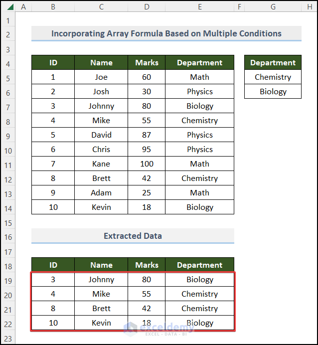
- Press Enter on your keyboard.
Later, you will get the first extracted data that matches your conditions in the result cell. E.g. Johnny whose ID is 3 is from the Biology department and his record is stored in the dataset first, so we got Johnny’s ID 3 in the result cell.
- Drag the Fill Handle from B19 to the entire result range to retrieve all details.
Read More: How to Extract Data From Table Based on Multiple Criteria in Excel
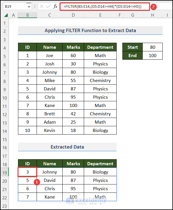
Method 3 – Applying FILTER Function to Extract Data Based on Criteria from Excel
Steps:
- Go to cell B19 and enter the following formula.
=FILTER(B5:E14,(D5:D14>=H4)*(D5:D14<=H5))Here, D5:D14 represents the range of Marks of the students.
- Press the Enter key.
Method 4 – Using Filter Option to Extract Data Based on Range Criteria from Excel
Steps:
- Select only the header of the dataset.
- Go to Data -> Filter.
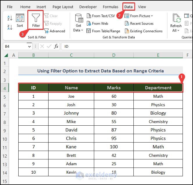
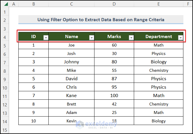
- This will insert a drop-down button in each header name of the dataset.
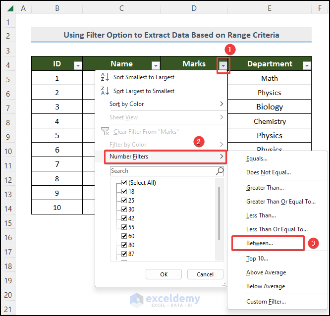
- Since we want to extract data based on the Marks, click on the drop-down button next to the Marks column.
- From the drop-down list, select Number Filters -> Between… (again, as we are extracting data between 80 to 100, we select the option Between. You can select any other options from the list according to your criteria).
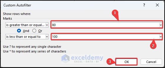
- From the pop-up Custom AutoFilter box, select 80 from the drop-down list which will appear by simply clicking on the drop-down button next to is greater than or equal to label, and select 100 in the label box is less than or equal to.
- Click OK.
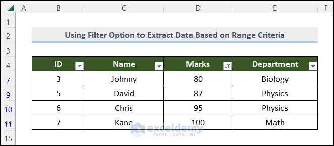
You will get all the details only for the students who got Marks from 80 to 100.
Read More: How to Extract Data from a List Using Excel Formula
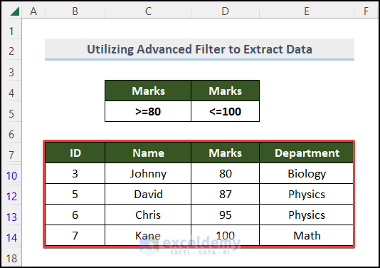
Method 5 – Utilizing Advanced Filter to Extract Data from Excel Based on Range Criteria
Steps:
- Select the entire data table.
- Go to Data, then to Advanced.
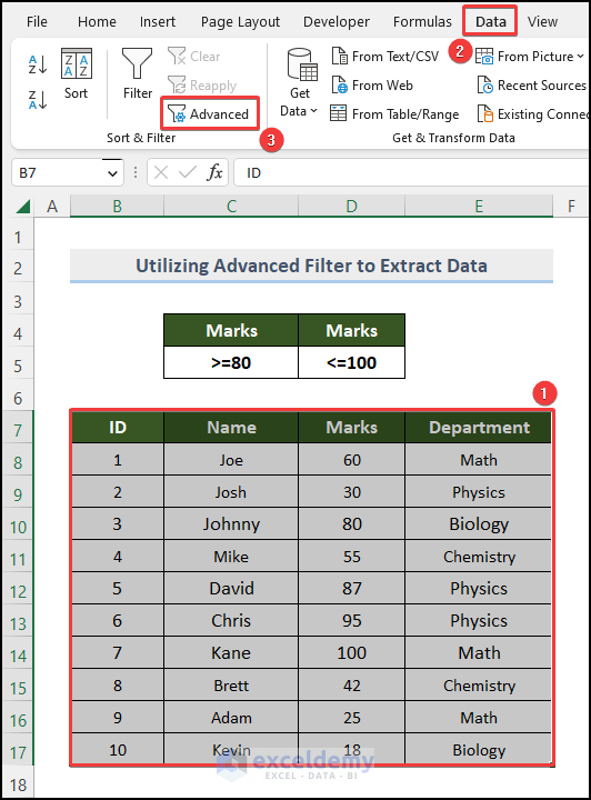
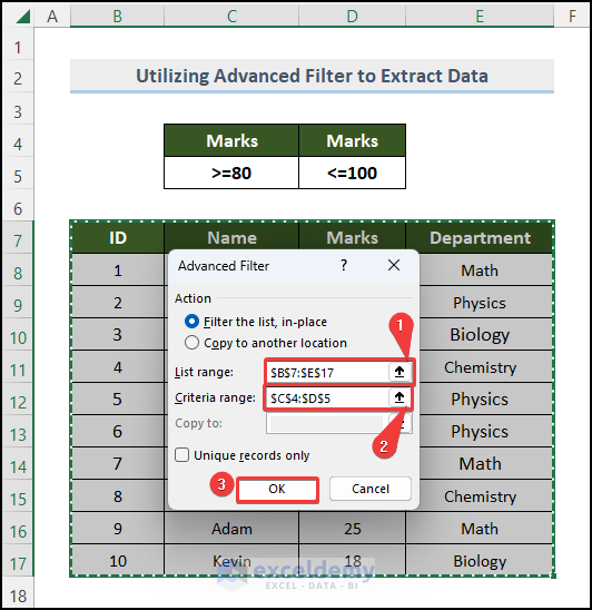
- You will see the range of your selected data in the box next to the List range option.
- In the box next to the Criteria range, select the cells carrying the defined conditions. You will see the name of the worksheet will be auto-generated there, following the cell reference numbers holding the predefined conditions.
- Click OK.
You will get all the details only for the students who got Marks from 80 to 100.
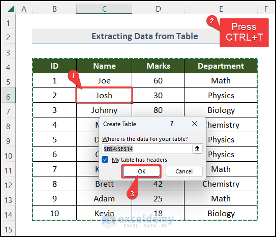
Method 6 – Extract Data from Excel-Defined Table Based on Range Criteria
Steps:
- Select any cell (we selected cell C6) from your dataset and press CTRL + T.
- A pop-up Create Table Box will appear, showing the range of your dataset as values. Keep the check box My table has headers marked.
- Click OK.
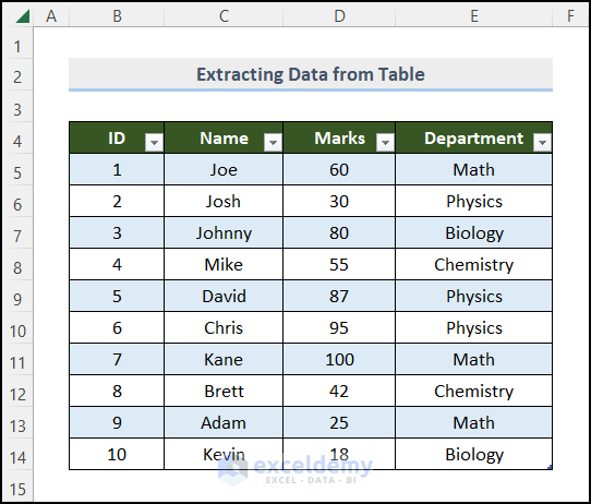
Excel will auto-generate a table based on your dataset with a drop-down button along with the headers.
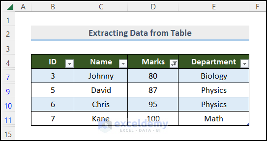
- Follow the steps shown in the previous method to get the desired output.
You will get an Excel-defined table carrying only the details of students’ who got Marks from 80 to 100.
Keep in Mind
- As the range of the data table array to search for the value is fixed, don’t forget to put the dollar ($) sign in front of the cell reference number of the array table.
- When working with array values, don’t forget to press CTRL + SHIFT + ENTER on your keyboard if you are working with any other version rather than Microsoft Excel 365.
- After pressing CTRL + SHIFT + ENTER, you will notice that the formula bar encloses the formula in curly braces {}, declaring it as an array formula. Don’t type those brackets {} yourself, Excel automatically does this for you.
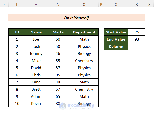
Practice Section
We have provided a Practice section like the one below where you can practice different filtering options.
Download Practice Workbook
You can download the free Excel practice workbook from here.
You May Also Like To Explore
- Excel Formula to Get First 3 Characters from a Cell
- How to Extract Month and Day from Date in Excel
- How to Extract Month from Date in Excel
- How to Extract Year from Date in Excel
<< Go Back To Extract Data Excel | Learn Excel
Get FREE Advanced Excel Exercises with Solutions!
