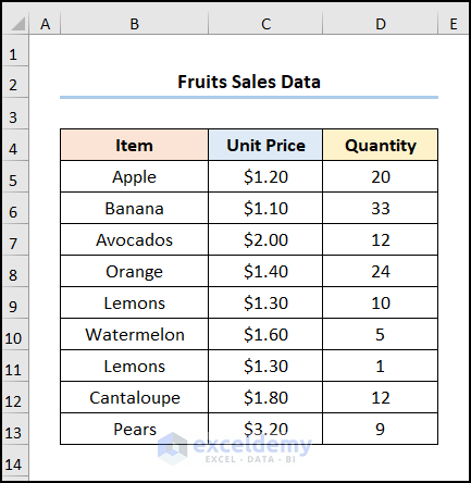
The sample dataset (B4:D13) showcases Item, Quantity, and Unit Price of Fruit Sales.
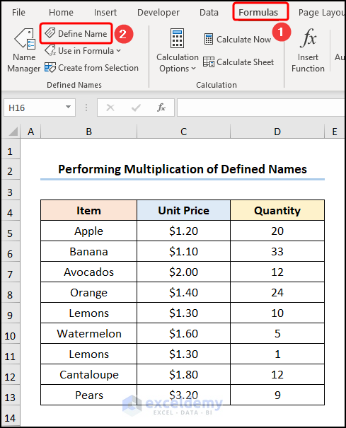
Example 1: Multiplying Named Ranges
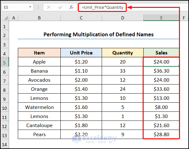
Multiply the “Unit Price” by “Quantity” to get the “Sales” in USD.
Steps:
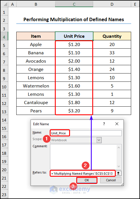
The Edit Name window will be displayed.
- In Name, enter “Unit_Price” >> in Refers to, select C5:C13 >> click OK to create a Defined Name.
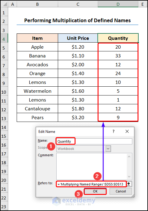
- Create a Defined Name for “Quantity” by selecting D5:D13.
- Multiply the “Unit Price” by “Quantity” to calculate the Sales in USD.
=Unit_Price*Quantity
The “Unit_Price” and the “Quantity” refer to the Defined Names: C5:C13 and D5:D13.
Note: In Microsoft 365, you can run the Array Formula by pressing ENTER. In older versions, you must press CTRL + SHIFT + ENTER.
Read More: How to Create a Formula in Excel without Using a Function
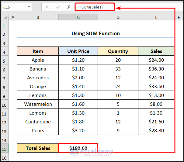
Example 2 –Using the SUM Function
Steps:
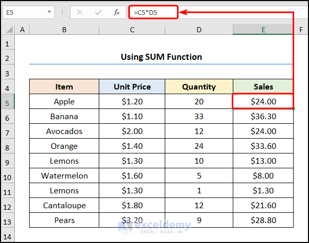
- Go to E5 >> enter the formula below.
=C5*D5
C5 and D5 cells represent “Unit Price” and “Quantity”.
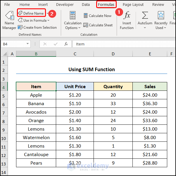
- Go to Formulas >> choose Define Name.
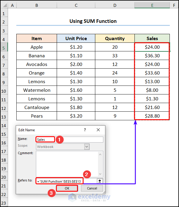
- Define a name (“Sales”) for E5:E13.
- Use the SUM function to obtain the “Total Sales” : “$190.60”.
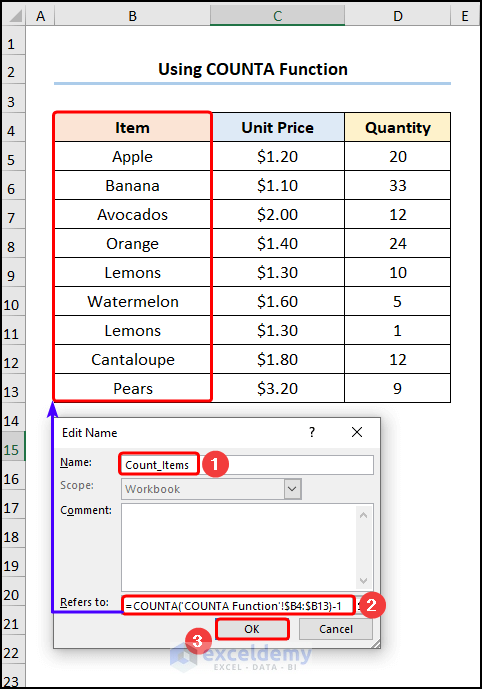
Example 3 – Utilizing the COUNTA Function
Use the COUNTA function.
Steps:
- Follow the steps described in the Example 2 >> Choose a name. Here, “Count_Items” >> insert the formula below.
=COUNTA('COUNTA Function'!$B4:$B13)-1
The ‘COUNTA Function’!$B4:$B13) is the value argument that represents the B4:B13 in the “COUNTA Function”.
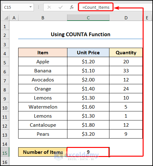
- Go to C15 >> enter the Defined Name “Count_Items” and press ENTER to see the count.
Note: You can open the list of Defined Names by pressing CTRL + F3.
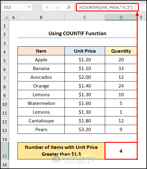
Example 4 -Using the COUNTIF Function
Use the COUNTIF function to count only those items that match the given criterion. You want to count the number of items with “Unit Price” exceeding “$1.5”.
Steps:
- Go to D15 >> Enter the formula.
=COUNTIF(Unit_Price,">1.5")
The “Unit_Price” points to the Defined Name which indicates C5:C13.
Formula Breakdown:
- COUNTIF(Unit_Price,”>1.5″) → counts the number of cells within a range that meet the given condition. Here, Unit_Price represents the range argument that refers to C5:C13, whereas the “>1.5” indicates the criteria argument that returns the count of the values greater than “$1.50”.
- Output → 4
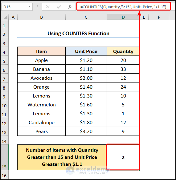
Example 5 – Applying the COUNTIFS Function
Combine the COUNTIFS function with the Defined Names Function to specify multiple criteria and return the instances that match the given condition. You want to see items in “Quantity” and “Unit Price” greater than “15” and “$1.1”.
Steps:
- Go to D15 >> Enter the formula in the Formula Bar.
=COUNTIFS(Quantity,">15",Unit_Price,">1.1")
“Quantity” and “Unit_Price” indicate the Defined Names.
Formula Breakdown:
- COUNTIFS(Quantity,”>15″,Unit_Price,”>1.1″) → counts the number of cells specified by a given set of conditions and criteria. Quantity represents the criteria_range1 argument that refers to D5:D13, whereas “>15” indicates the criteria1 argument that represents the condition greater than “15”. Unit_Price represents the criteria_range2 argument that refers to C5:C13, whereas “>1.1” indicates the criteria2 argument that represents the condition greater than “$1.1”.
- Output → 2
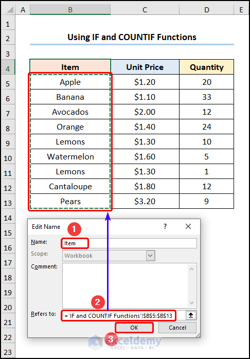
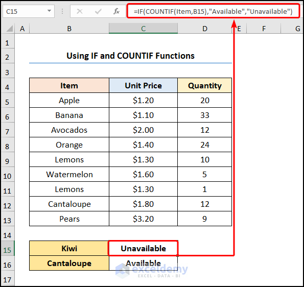
Example 6 – Combining the IF and the COUNTIF Functions
Use the IF and COUNTIF functions to check if the name of the fruit is present within the list.
Steps:
- Follow the steps described in example 5 to create a Defined Name for “Item”.
- In C15, enter the formula below.
=IF(COUNTIF(Item,B15),"Available","Unavailable")
B15 cell indicates “Kiwi”.
Formula Breakdown:
- COUNTIF(Item,B15) → Item represents the range argument that refers to the Item column, whereas B15 indicates the criteria argument:“Kiwi”. Since “Kiwi” is not present, the function returns zero, which implies FALSE.
- Output → 0
- IF(COUNTIF(Item,B15),”Available”,”Unavailable”) → becomes
- IF(0,”Available”,”Unavailable”) → checks whether a condition is met and returns one value if TRUE and another value if FALSE. Here, 0 is the logical_test argument, which prompts the IF function to return “Unavailable” (value_if_false argument), otherwise, “Available” (value_if_true argument).
- Output → Unavailable
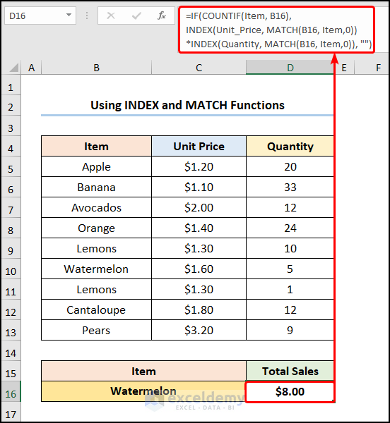
Example 7 – Using the INDEX and the MATCH Functions
Use the INDEX, and MATCH functions to calculate the “Total Sales” based on a selected “Item”.
Steps:
- Go to D16 >> Enter the following formula
=IF(COUNTIF(Item, B16),INDEX(Unit_Price, MATCH(B16, Item,0))*INDEX(Quantity, MATCH(B16, Item,0)), "")
B16 refers to the “Watermelon”.
Formula Breakdown:
- MATCH(B16, Item,0) → returns the relative position of an item in an array matching the given value. B16 is the lookup_value argument that refers to “Watermelon”. Item represents the lookup_array argument from which the value is matched. 0 is the optional match_type argument which indicates Exact match criteria.
- Output → 6
- INDEX(Unit_Price, MATCH(B16, Item,0)) → becomes
- =INDEX(Unit_Price, 6) → returns a value at the intersection of a row and column in a given range. Unit_Price is the array argument. 6 is the row_num argument that indicates the row location.
- Output → $1.6
- IF(COUNTIF(Item, B16),INDEX(Unit_Price, MATCH(B16, Item,0))*INDEX(Quantity, MATCH(B16, Item,0)), “”) → becomes
- IF(1,1.6*5,””) → 1 is the logical_test argument which prompts the IF function to return 1.6*5 (value_if_true argument). Otherwise, it returns “” (Blank) (value_if_false argument).
- Output → $8.00
Read More: How to Create a Complex Formula in Excel
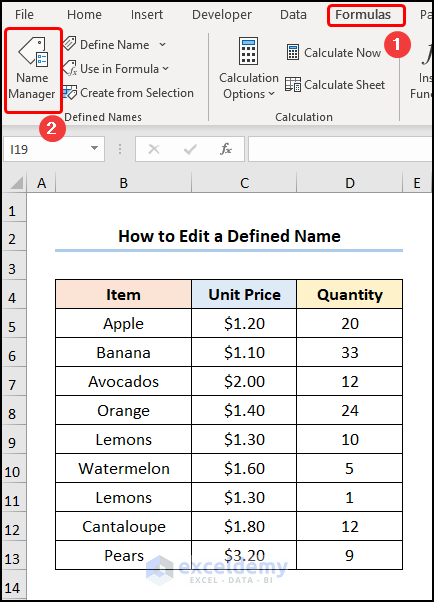
How to Edit a Defined Name in Excel
Steps:
- Go to the Formulas tab >> choose Name Manager.
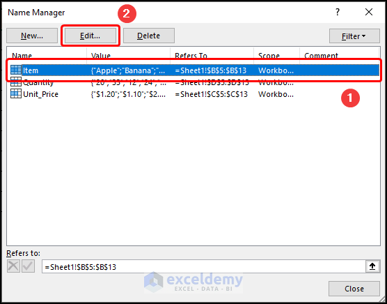
- Select a Defined Name, here “Item” >> Click Edit.
- Rename the range or enter a different range.
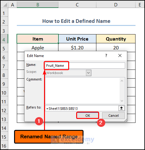
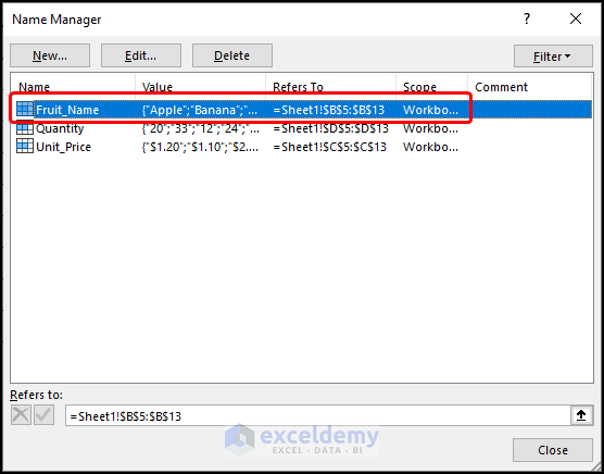
This is the output.
How to Delete Defined Names in Excel
Steps:
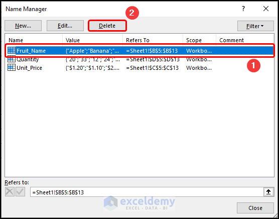
- Go to the Formulas tab >> select Name Manager.
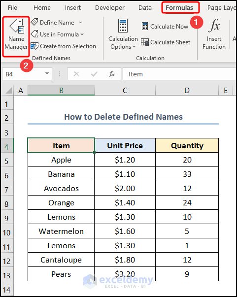
- Select the Defined Name. Here, “Fruit_Name” >> Click Delete.
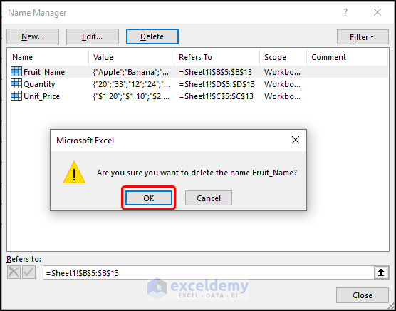
Click OK to delete the Defined Name.
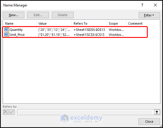
This is the output.
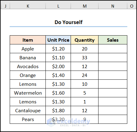
Practice Section
Practice here.
Download Practice Workbook
Related Articles
- How to Create a Formula in Excel for Multiple Cells
- How to Create a Custom Formula in Excel
- How to Apply Formula in Excel for Alternate Rows
- How to Insert Formula for Entire Column in Excel
- How to Create a Conditional Formula in Excel
<< Go Back to How to Create Excel Formulas | Excel Formulas | Learn Excel
Get FREE Advanced Excel Exercises with Solutions!
