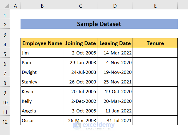
We will use the following dataset to demonstrate 5 easy methods to calculate tenure in years and months in Excel. In the dataset below, you see the Joining Date and Leaving Date of several employees. We will try to calculate their tenure.
Method 1 – Apply the DATEDIF Function to Calculate Tenure in Years and Months
In this article, we will learn 5 easy methods to calculate tenure in years and months in Excel. We will use the following dataset to demonstrate these methods. In the following dataset, we have shown the Joining Date and Leaving Date of some employees. Now we will calculate their tenure.
1. Apply DATEDIF Function to Calculate Tenure in Years and Months
This is the most convenient method to calculate tenure in years and months in Excel. We will use the DATEDIF function for this purpose. Follow the steps to calculate tenure using the DATEDIF function.
Steps:
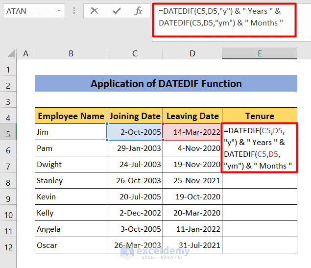
- Enter the following formula in cell E5:
=DATEDIF(C5,D5,"y") & " Years " &DATEDIF(C5,D5,"ym") & " Months "- C5 refers to the joining date and D5 refers to the leaving date.
- DATEDIF(C5,D5,”y”) returns the number of years in integer form after subtracting the leaving date of D5 from the joining date C5.
- DATEDIF(C5,D5,”ym”) returns the number of months for the fraction value of years.
- Press Enter. The desired result is shown in cell E5.
- Drag the bottom right corner of cell E5 to E12 by holding the left button of the mouse.
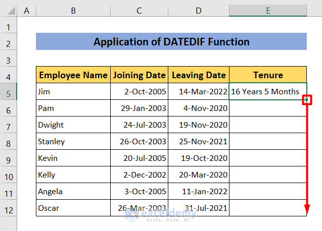
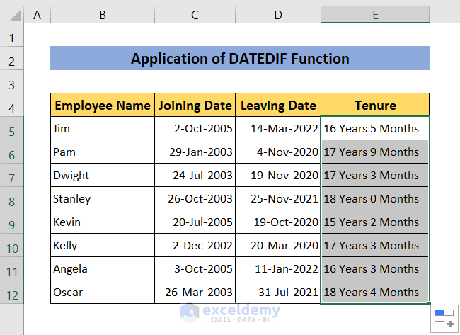
- You will get the values of years and months for all the dates.
Read More: Calculate Years and Months Between Two Dates in Excel
Method 2 – Insert the LET Function to Calculate Tenure in Years and Months
In this method, we will use the LET function to show another way to calculate tenure in years and months.
Steps:
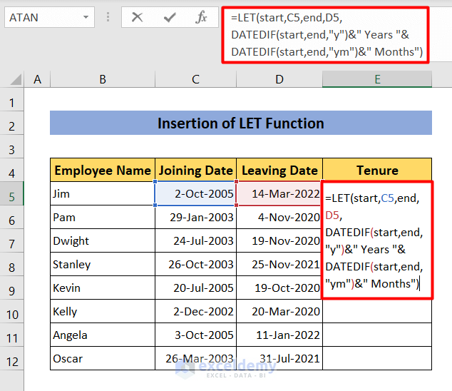
- Enter the following formula in cell E5:
=LET(start,C5,end,D5,DATEDIF(start,end,"y")&" Years "&DATEDIF(start,end,"ym")&" Months")- In the formula, C5 and D5 refer to the joining and leaving dates, respectively.
- LET(start,C5,end,D5) assigns the name start for cell C5 and end for cell D5.
- DATEDIF(start,end,”y”)&” Years “&DATEDIF(start,end,”ym”)&” Months”) looks into the start date and end date and returns tenure value in years and months.
- Hit Enter to see the result in cell E5.
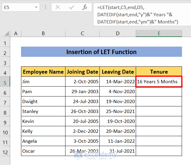
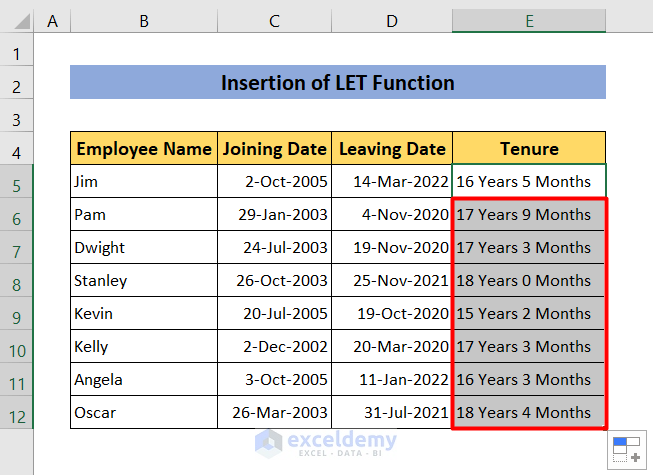
- To see the results for all the data, just double-click the bottom right corner of cell E5.
- It will show the results in years and months format.
Read More: How to Calculate Years Between Two Dates in Excel
Method 3 – Combine the INT and ROUND Functions to Calculate Tenure in Years and Months
Steps:
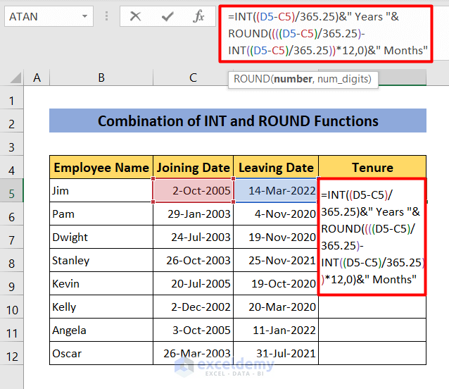
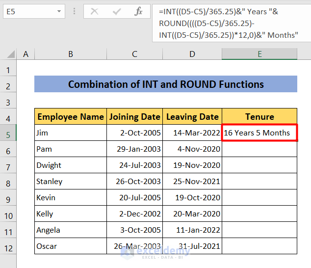
- Enter the following formula in cell E5:
=INT((D5-C5)/365.25)&" Years "& ROUND((((D5-C5)/365.25)- INT((D5-C5)/365.25))*12,0)&" Months"- INT((D5-C5)/365.25 subtracts the date from cell D5 to C5. Then it divides the value by 365.25 and returns years in integer format. In cell E5, it returns 17 years.
- ROUND((((D5-C5)/365.25)- INT((D5-C5)/365.25))*12,0) multiplies the fraction part of the year and round it off to return the value of months. In cell E5, it returns 5 months.
- Press Enter to get the result.
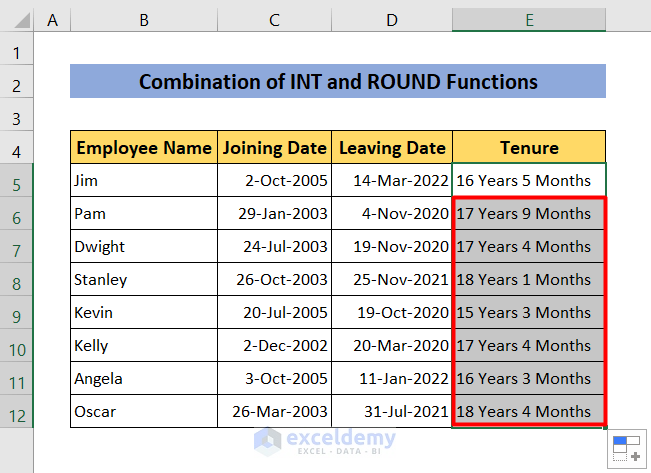
- Double-click the bottom right corner of cell E5 and see the results for all the dates.
Read More: How to Calculate Remaining Days in Excel
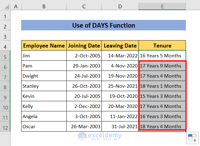
Method 4 – Use the DAYS Function to Calculate Tenure in Years and Months
Steps:
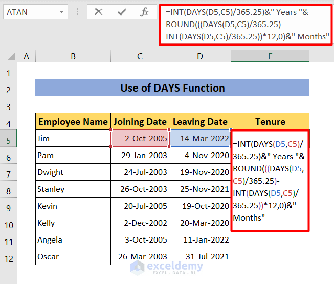
- Enter the following formula in cell E5:
=INT(DAYS(D5,C5)/365.25)&" Years "& ROUND(((DAYS(D5,C5)/365.25)- INT(DAYS(D5,C5)/365.25))*12,0)&" Months"- INT(DAYS(D5,C5)/365.25) divides the number of days by 365.25 and returns the results in integer format.
- ROUND(((DAYS(D5,C5)/365.25)-INT(DAYS(D5,C5)/365.25))*12,0) multiplies the fraction part of the year and rounds it off to return the value of months.
- Hit Enter to get the tenure in years and months.
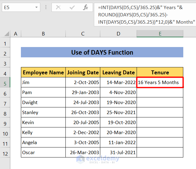
- To get the results for all the data, move the cursor at the bottom right corner and click the left button of the mouse twice.
Read More: How to Calculate Average Tenure of Employees in Excel
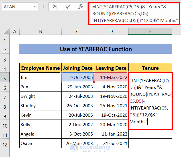
Method 5 – Utilize YEARFRAC Function to Calculate Tenure in Years and Months
Steps:
- Enter the following formula in cell E5:
=INT(YEARFRAC(C5,D5))&" Years "& ROUND((YEARFRAC(C5,D5)- INT(YEARFRAC(C5,D5)))*12,0)&" Months"- INT(YEARFRAC(C5,D5)) returns the number of years between the date of C5 and D5 in integer format.
- ROUND((YEARFRAC(C5,D5)-INT(YEARFRAC(C5,D5)))*12,0) multiplies the fraction part of the year and rounds it off to return the value of months.
- Press Enter. Years and months of tenure will be shown in cell E5.
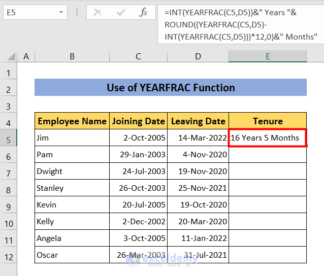
- To calculate tenure for all the employees, click the bottom right corner of cell E5 twice.

Things to Remember
- While using a formula, don’t forget to give proper cell references or you won’t get the desired results.
- Be careful about using the parenthesis while writing any formula. Parenthesis in the wrong position might show the wrong results.
Download Practice Workbook
Download this practice workbook for practice while you are reading this article.
Related Articles
- How to Calculate Overdue Days in Excel
- How to Calculate Working Capital Days in Excel
- How to Calculate Days Outstanding in Excel
- How to Calculate 90 Days from a Specific Date in Excel
- How to Create a Day Countdown in Excel
<< Go Back to Days Between Dates | Date-Time in Excel | Learn Excel
Get FREE Advanced Excel Exercises with Solutions!
