How Do You Link Sheets in Excel with Index (3 Swift Ways)

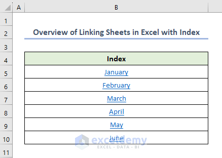
In this article, we are going to show you how you link sheets in Excel with an index. We will apply the HYPERLINK link function, VBA macro, and also use the Hyperlink dialog box to link up sheets in Excel with an index.

Linking sheets in Excel is a powerful feature that allows you to connect and consolidate data from multiple worksheets within a workbook or even across different workbooks. By establishing these connections, you can create dynamic relationships between sheets, enabling efficient data management and analysis.

Knowing how to link sheets properly may dramatically improve your productivity and optimize your workflow, whether you’re working on complicated financial models, tracking project progress, or organizing data for reporting reasons.

Download Practice Workbook

If you want a free copy of the illustrated workbook we discussed during the presentation, please click the link below this section.

How Do You Link Sheets in Excel with Index: 3 Swift Ways

Now let’s explore three easy ways to link sheets with index with proper steps and illustrations.

1. Using Insert Hyperlink Dialog Box to Link Sheets with Index

Here we will show you how to link worksheets with an index by using the Insert Hyperlink dialog box. Let’s follow the following instructions to link up the worksheets:

• Select cell B5 and then press CTRL+K.

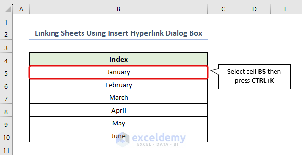
• A dialog box like the below image will appear before you.
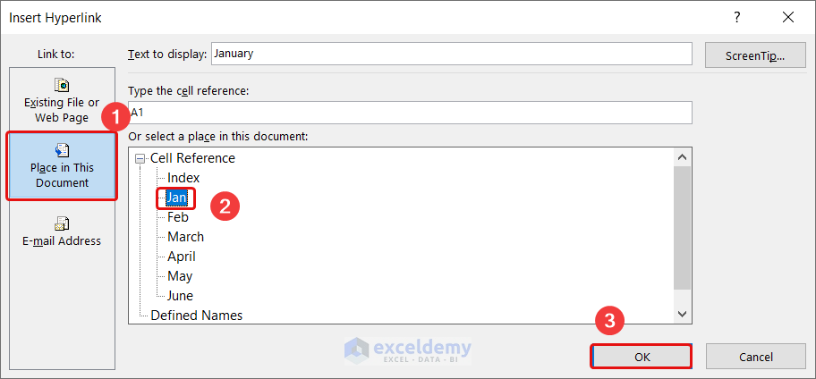
• From the dialog box select Place in This Document >> Jan.
• Then press OK.

For a better understanding take a look at the following image.

You can add hyperlinks to other worksheets by doing this process.  Do this for the other cells from B6 to B10 and the output will look like the image below.

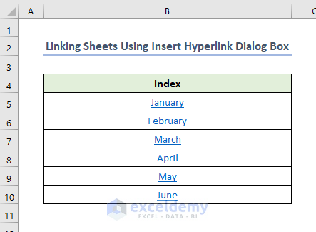
If you click on cell B5 you will go to the worksheet Jan. See the gif below for a better idea.

2. Using Excel Formula to Link Sheets with Index

We can also link a worksheet by using the Excel formula. We will use the HYPERLINK function to link the worksheets. Now, follow the steps below:

• Select cell B5 and write down the following formula.

• Then press Enter.

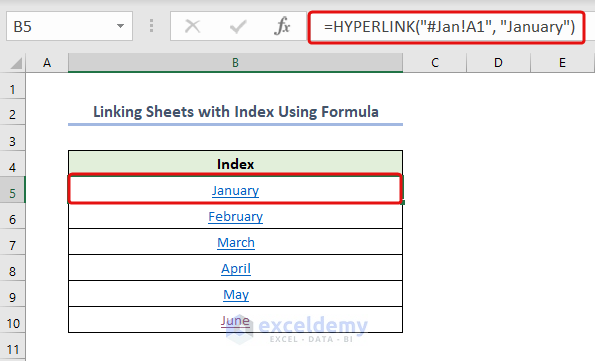
• HYPERLINK is an Excel function that creates a hyperlink. #Jan!A1 is the link target or URL of the hyperlink. In this case, it is “#Jan!A1“. The #(hash) symbol refers to the same document or workbook, and Jan is the name of a worksheet in the workbook. A1 refers to cell A1 in the worksheet. “January” is the text or display value of the hyperlink. It is the clickable text that appears in the cell or on the worksheet.

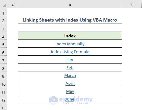
3. Creating Hyperlinked Index of Sheets Using VBA Macro

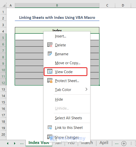
In this segment, we will use VBA macro to link all the worksheets of your workbook and also create a hyperlinked index. Let’s follow the guidelines below for linking the worksheets in the index:

• Select the worksheet name and then right-click on your mouse.
• Then select View code from the context menu.

• A worksheet window of VBA will open.
• Paste the following code in the worksheet window and then click on the play button or press F5.

Private Sub Worksheet_Activate()
    'Defining variables
    Dim sheet As Worksheet
    Dim row As Long
    row = 4
    'Using the worksheet name, loop over each page to add a relevant hyperlink.
    For Each sheet In Worksheets
        If sheet.Name <> Me.Name And sheet.Visible = xlSheetVisible Then
            row = row + 1
            Me.Hyperlinks.Add Anchor:=Me.Cells(row, 2), _
             Address:="", _
             SubAddress:="'" & sheet.Name & "'!A1", _
             ScreenTip:="Click to go to sheet " & sheet.Name, _
             TextToDisplay:=sheet.Name
        End If
    Next sheet
    Me.Columns(1).AutoFit
End Sub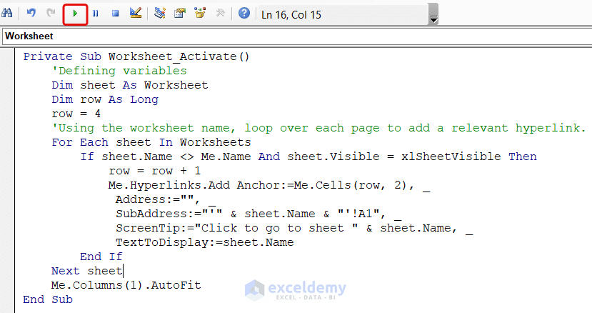

After executing the code, you will see the output like the image below. You can go to any worksheet by clicking on the worksheet name from the index.

Note: This code won’t run on the module. So, you have to run it on the worksheet as we stated above.

Things to Remember

• Sheet Names: Ensure that you know the names of the sheets you want to link. Double-check the spelling and ensure they are accurate. Excel is case-insensitive, but it’s still good practice to use the correct capitalization.
• Updating Links: If you later change the sheet name or move the referenced sheet to a different location, the links may break. Excel will display a #REF! error if the linked sheet cannot be found. Double-check your links if you encounter this error.
• Cell references: When linking sheets, you need to specify the correct cell references. Ensure that you reference the correct sheet name followed by an exclamation mark (!) before specifying the cell or range of cells. For example, to link to cell A1 in Sheet2, you would use “=Sheet2!A1“.

Frequently Asked Questions

1. Can I move or copy linked sheets within a workbook?

Yes, when you move or copy sheets within the same workbook, Excel automatically updates the formulas and links to reflect the new sheet location. However, check for absolute references ($A$1) that may still refer to the original sheet.

2. What happens if I rename or delete a linked sheet?

If you rename or delete a linked sheet, the link will break. Excel displays a warning message and shows the old sheet name as a placeholder. You need to update the formula with the correct sheet name or fix the link. But if you use VBA then it may update automatically.

3. How do I link sheets in different workbooks?

To link sheets in different workbooks, include the complete file path along with the sheet name. For example, “=C:\FolderName[WorkbookName.xlsx]SheetName!A1″. Ensure the referenced workbook is accessible and the path is correct.

Conclusion

After going through the article, you have a comprehensive idea of linking sheets in Excel with an index. You may create reliable links that dynamically update as your data changes by knowing how to use cell references, sheet names, and file locations properly.

I hope you like this article. If you have any suggestions or queries regarding this article, then post your valuable comments in the comment section below and do visit the ExcelDemy website to explore more Excel functions and features.