Method 1 – Using the RANDARRAY Function
The RANDARRAY function, introduced in Excel 365, generates arrays of random numbers.
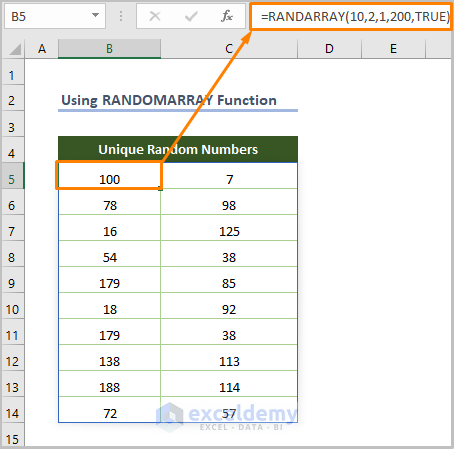
For example, if you want 20 unique random numbers between 1 and 200, you can use this formula:
=RANDARRAY(10,2,1,200,TRUE)
Here’s what each part of the formula means:
- 10 is the number of rows (how many numbers you want).
- 2 is the number of columns (usually you only need 1).
- 1 is the minimum value (in this case, 1).
- 200 is the maximum value (in this case, 200).
- TRUE tells the function to give you whole numbers (integers).
Note: This method works best when you only need a small number of unique random numbers from a large range (e.g. generating 10/20 numbers from 1 to 200/500). If you need a lot of random numbers close together, you might get some duplicates.
Method 2 – Using UNIQUE & RANDARRAY Functions
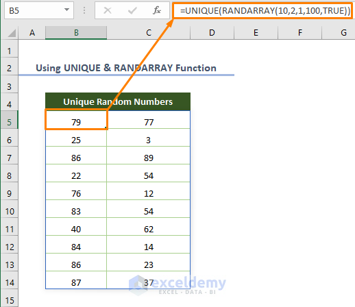
The UNIQUE function, available in Excel 365 and Excel 2021 versions, returns a list of unique values from a given dataset or cell range. UNIQUE function can be combined with RANDARRAY function to produce random numbers without repetition.
Here’s an example formula:
=UNIQUE(RANDARRAY(10,2,1,100,TRUE))
This formula does the same thing as the previous one, but it uses the UNIQUE function to make sure there are no repeats.
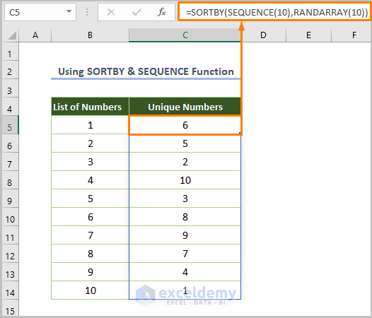
Method 3 – Applying SORTBY & SEQUENCE Functions to Generate Random Number with No Repeats
The SEQUENCE function, accessible only in Excel 365 & Excel 2021 versions, produces a list (array) of sequential numbers.
Here’s an example formula to get 10 unique random numbers between 1 and 10:
=SEQUENCE(10)
Here, 10 is the number of rows.
Next, the SORTBY function sorts an array of values based on another array of values with ascending or descending order. Hence, we may use the function along with the SEQUENCE & RANDARRAY function to create 10 random numbers without repetition.
=SORTBY(SEQUENCE(10),RANDARRAY(10))
This formula works like this:
- RANDARRAY(10) makes a list of 10 random numbers.
- SEQUENCE(10) makes a list of 10 sequential numbers.
- SORTBY sorts the list of numbers in order based on the random order of the first list.
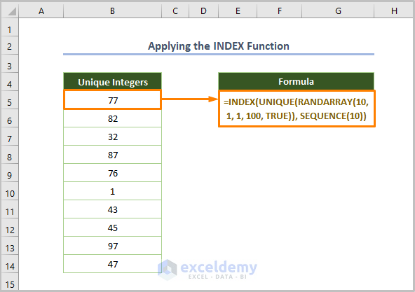
Method 4 – Utilizing the INDEX Function as Random Number Generator with No Repeats
You can use the INDEX function along with the previously discussed RANDARRAY, SEQUENCE & UNIQUE functions to produce 4 types of random numbers.
4.1. Producing Random Integer Numbers
Use the following formula to get 10 random integers between 1 and 100 without repetition.
=INDEX(UNIQUE(RANDARRAY(10, 1, 1, 100, TRUE)), SEQUENCE(10))
This formula works like this:
- SEQUENCE(10) creates 10 sequential numbers,
- RANDARRAY(10, 1, 1, 100, TRUE) produces 10 random integer numbers between 1 and 100.
- TRUE is used for generating integer numbers.
- UNIQUE function removes the repetitive values from the generated numbers.
- INDEX function returns the 10 random integer numbers as directed by the SEQUENCE function.
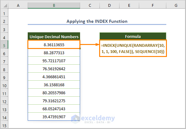
4.2. Producing Random Decimal Numbers
To generate 10 random decimal numbers without repetition, use the following formula.
=INDEX(UNIQUE(RANDARRAY(10, 1, 1, 100, FALSE)), SEQUENCE(10))
Here, 10 is the number of rows, 2 is the number of columns, 1 is the minimum value, 100 is the maximum value, and FALSE is for generating decimal numbers.
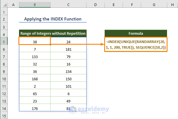
4.3. Producing a Range of Integer Numbers
Generate a range of random integers using the following formula.
=INDEX(UNIQUE(RANDARRAY(20, 1, 1, 200, TRUE)), SEQUENCE(10,2))
Here, 20 is the number of rows, 1 is the number of columns, 1 is the minimum value, 200 is the maximum value, and TRUE is for generating integer numbers.
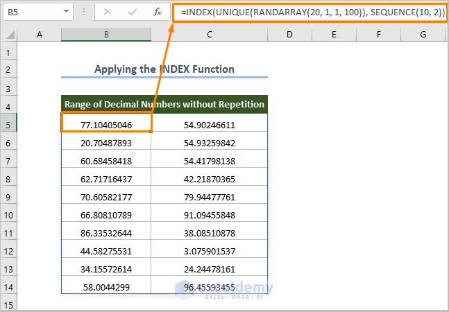
4.4. Producing a Range of Random Decimal Numbers
For generating a range of random decimal numbers between 1 and 100, use the following formula.
=INDEX(UNIQUE(RANDARRAY(20, 1, 1, 100)), SEQUENCE(10, 2))
Here, 20 is the number of rows, 1 is the number of columns, 1 is the minimum value, 200 is the maximum value, and FALSE is for generating decimal numbers.
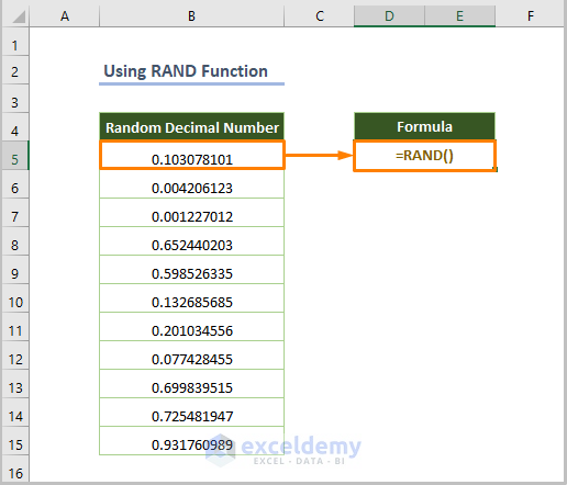
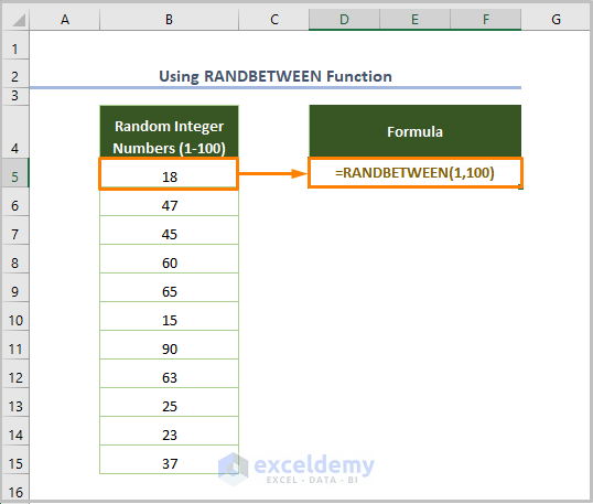
Method 5 – RAND & RANDBETWEEN Functions to Generate Random Number
The RAND function generates a number between 0 to 1. Use the formula if you want to generate unique decimal numbers.
=RAND()
The RANDBETWEEN function gives random numbers between two given numbers.
For example, if you want to get the integer numbers between 1 and 100, you can use the formula below.
=RANDBETWEEN(1,100)
Here, 1 is the bottom argument and 100 is the top argument.
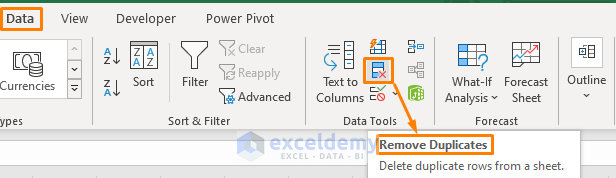
There’s a higher chance of getting duplicates while using the RANDBETWEEN function, but you can use the Remove Duplicates option from the Data tab in the Data Tools ribbon after selecting the cell range.
Method 6 – Applying RAND & RANK Functions as Random Number Generator
Furthermore, you can use the RANK function which returns the relative size of a number based on the given list of numbers. Before doing that create a list of random decimal numbers utilizing the RAND function.
=RANK(B5,$B$5:$B$15)
Here, B5 is the starting cell of decimal numbers and B5:B15 is the cell range for decimal numbers.
![]()
Method 7 – Utilizing the Combination of RANK.EQ & COUNTIF Functions
Let’s say you want to generate random numbers without repetition from 10 to 50.
First, create a list of numbers between 10 and 50 using the RANDBETWEEN function.
Now, use the formula below-
=9+RANK.EQ(B5, $B$5:$B$15) + COUNTIF($B$5:B5, B5) - 1
Here, B5 is the starting cell of random numbers and B5:B15 is the cell range for decimal numbers.
The COUNTIF function is counting each random number that is available in the list. RANK.EQ returns the relative position (rank) for each random number. 9 is added because we want to generate the number starting from 10.
![]()
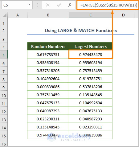
Method 8 – LARGE & MATCH Functions as Random Number Generator in Excel
We can produce random integer numbers without repetition using the combination of the LARGE and MATCH functions. The LARGE function returns the kth largest value in a given cell range or dataset.
=LARGE($B$5:$B$15,ROW(B1))
Here, $B$5:$B$15 is the cell range for random decimal numbers that are found using the RAND function, ROW(B1) refers to row number 1.
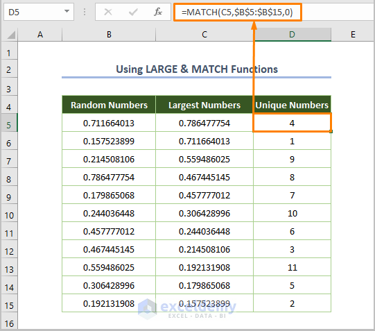
Use the following formula to find the position of the created largest value.
=MATCH(C5,$B$5:$B$15,0)
Here, C5 is the starting cell of the largest numbers, $B$5:$B$15 is the cell range of random decimal numbers, and 0 is for getting an exact match.
Method 9 – Analysis Toolpak as Random Number Generator in Excel
If you don’t like using formulas, you can use an Excel add-in called the Analysis ToolPak. This add-in has a random number generator that can create unique random numbers.
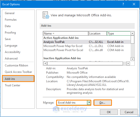
To use the Add-ins, follow the steps below.
⇰ Go to File > Options.
⇰ Click on the Add-ins and select Excel Add-ins from the drop-down list and pick the option Go.
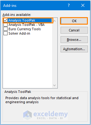
⇰ In the Add-ins dialog box, check Analysis ToolPak and press OK.
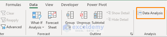
⇰ Select the Data Analysis option from the Data tab in the Analysis ribbon.
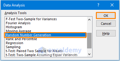
⇰ Choose the option Random Number Generation and press OK.
⇰ In the dialog box choose the options based on your desired output.
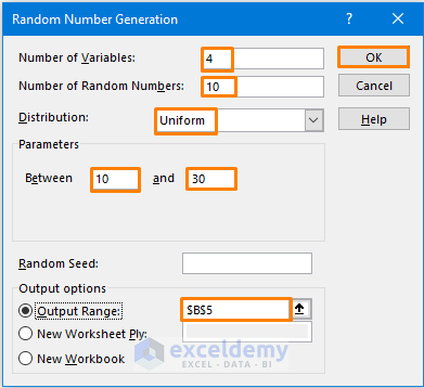
⇰ For example, I selected Number of Variables and Number of Random Numbers as 4 & 10 respectively to generate the list of numbers having 10 rows and 4 columns.
⇰ Select the Distribution as Uniform to avoid repetitive values.
⇰ Between 10 and 30 means I want to find the number within the range.
⇰ Select the Output Range and click OK
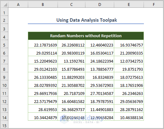
Your output will be generated.
Some Common Errors
There are a few errors you might run into when using these formulas.
| Name of Error | Cause of error |
|---|---|
| #CALC! | If the UNIQUE function cannot extract the unique values. |
| #SPILL! | If there is any value in the spill range where the UNIQUE function will return the list. |
| #VALUE! | The RANDARRAY function occurs when the minimum value is larger than the maximum value. |
Download Practice Workbook
<< Go Back to Random Number in Excel | Randomize in Excel | Learn Excel
Get FREE Advanced Excel Exercises with Solutions!

great thanksssssssssss Mr Md