Depreciation is described as the continual lowering of a fixed asset’s reported cost until the asset’s value is zero or insignificant. We can easily design a simple fixed asset depreciation calculator using Microsoft Excel. In this article, we are going to demonstrate 3 basic methods to create a fixed asset depreciation calculator in Excel. If you are also curious about it, download our practice workbook and follow us.
Overview of Depreciation Methods
Depreciation is described as the continual lowering of a fixed asset’s reported cost until the asset’s value is zero or insignificant. We can estimate the value of any fixed asset’s depreciation value using three methods.
- Straight-Line Method
- Unit of Production Method
- Double Declining Balance Method
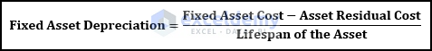
Straight-Line Method: The most straightforward depreciation calculation method is the straight-line method. In this method, the depreciation value is the ratio of the difference between the fixed asset cost and the asset’s residual cost, and the lifespan of that asset. Thus, we can show the mathematical expression as,
Unit of Production Method: In this case, the depreciation value is the multiplication value of the yearly production unit and the ratio of the difference between the fixed asset cost and the asset’s residual cost, and the total production unit of the asset’s lifespan. The formula can be shown below:

Double Declining Balance Method: According to this method, the depreciation value is the ratio of 2 times the difference between the fixed asset cost and the asset’s residual cost and the lifespan of that asset. The mathematical formula of this method is,

To demonstrate the methods, we consider a dataset of a sample asset. The cost of that fixed asset is $10,000,000. Its lifespan is 15 years, and after 15 years, its residual cost will be $10,000.
📚 Note:
All the operations of this article are accomplished by using Microsoft Office 365 application.
1. Using Straight-Line Method
In the first method, we are going to use the Straight-Line method to create a fixed asset depreciation calculator in Excel. Our fixed asset’s specification is in the range of cells C5:C8. We will display the depreciation value in cell C10.

The steps of this approach are given below:
📌 Steps:
- First of all, select cell C10.
- Now, write down the following formula in the cell.
=(C5-C7)/C6
- Press Enter.
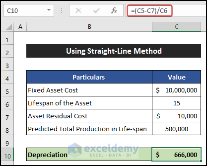
- You will get depreciation value.
Thus, we can say that our formula works perfectly, and we are able to create a fixed asset depreciation calculation by the Straight-Line method.
Read More: Create Depreciation Schedule in Excel
2. Applying Unit of Production Method
In this method, we will estimate the depreciation value by the Unit of Production method. Besides the previous specifications, to follow this project, we need the approximate amount of production for the first and second years. Both values are shown in the range of cells C9:C10. We will display the results in the range of cells C13:D13.

The steps of this process are given as follows:
📌 Steps:
- First, select cell C13.
- After that, write down the following formula in the cell.
=((C5-C7)/C8)*C9
- Then, press Enter.
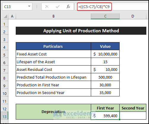
- You will get the depreciation value which will reduce after passing the first year.
- Similarly, select cell D13.
- Afterward, write down the following formula inside the cell.
=((C5-C7)/C8)*C10
- Again, press Enter.
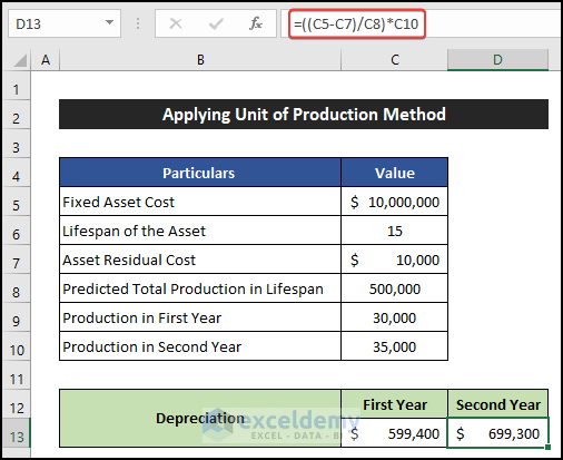
- In this way, you will be able to calculate the depreciation value for each year.
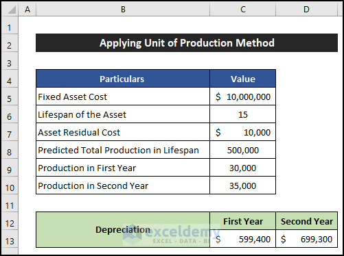
Hence, we can say that both formulas work effectively, and we are able to create a fixed asset depreciation calculation by the Unit of Production method.
Read More: How to Create Vehicle Depreciation Calculator in Excel
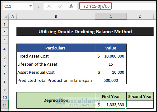
3. Utilizing Double Declining Balance Method
In the last method, we are going to use the Double Declining Balance method to design a fixed asset depreciation calculator in Excel. We will use our previous dataset to demonstrate this process. The result will be in the range of cells C13:D13.

The procedure of the method is explained below step-by-step.
📌 Steps:
- Firstly, select cell C13.
- Next, write down the following formula in the cell. In the first year, we don’t have any depreciation value for the last year. Hence, the value of the Accumulated Depreciation will be zero (0).
=(2*(C5-0))/C6
- Now, press Enter.
- Again, select cell D13 and write down the following formula in the cell. Here, the value of the Accumulated Depreciation will be the value of the depreciation value of the first year.
=(2*(C5-C11))/C6
- Similarly, press Enter.
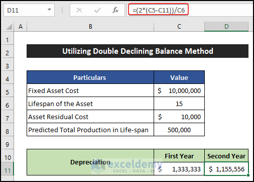
- You will be able to determine the depreciation value for each year.
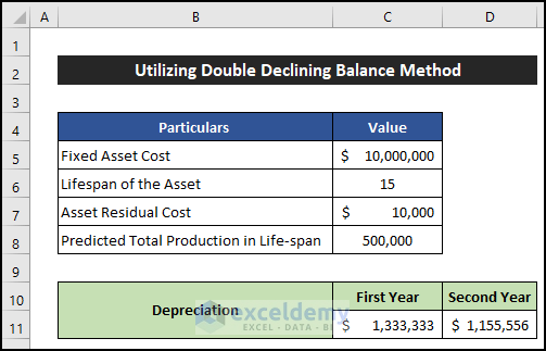
Finally, we can say that both formulas work successfully, and we are able to create a fixed asset depreciation calculation by the Double Declining Balance method.
Download Practice Workbook
Download this practice workbook for practice while you are reading this article.
Conclusion
That’s the end of this article. I hope that this article will be helpful for you and you will be able to create a fixed asset depreciation calculator in Excel. Please share any further queries or recommendations with us in the comments section below if you have any further questions or recommendations.
Keep learning new methods and keep growing!
Related Articles
- How to Create Monthly Depreciation Schedule in Excel
- How to Create Rental Property Depreciation Calculator in Excel
<< Go Back to Depreciation Template | Finance Template | Excel Templates
Get FREE Advanced Excel Exercises with Solutions!
